`Bitcoin Price Forecasting`¶

Milestone Project 3¶

The goal of this notebook is to explore time series forecasting by predicting Bitcoin prices (BitPredict)

What is a time series problem?¶

Time series deals with data over time:

Predicting weather (short term and medium term forecasts), climate (long term forecasts)
Predicting sales accross different geographies for different products in the catalog (might require a bit of geostatistics)
Identifying special events in time, such as anomalies:
- Anomalous weather events (maybe temperature at different pressure levels is changing), SST anomalies in the equitorial pacific ocean
- Sensor data anomalies in an aircraft, consisting of thousands of sensors

The problems can be broadly categorized into two categories:

Problem Type	Examples	Output
Classification	Anomaly detection, time series identification (where did this time series come from?)	Discrete (a label)
Forecasting	Predicting stock market prices, forecasting future demand for a product, stocking inventory requirements	Continuous (a number)

Contents of this Notebook¶

Acquire the bitcoin time series data csv file
Format data for time series problem
- Split into training and test sets the wrong way
- Split into training and test sets the right way
- Visualizing the data
- Converting time series forecasting into a supervised learning task
- Preparing univariate and multivariate time series data
Evaluate a time series forecasting model
- Generally, this would depend on how much ahead forecast we are evaluating. 1-day error, 2-day error
- Evaluation methods can be done for models which are trained differently. For e.g. we train a 3 window 1 horizon model 1, and 7 window 2 horizon model 2, and we want to evaluate the 2 day forecast error rate. In this case for model 1, we would have to forecast recursively to get the 2 day ahead. forecast
Setting up different deep learning modelling experiments:
- Dense models
- Sequence models (CNN/LSTM)
- Ensembling methods
- Multivariate models
- Re-implementing the N-BEATS algorithm using Tensorflow
Creating modelling checkpoints to save the best model
Forecasting using a time series model
Estimation of prediction confidence intervals (quantifying forecast uncertainty)
Discussing two types of uncertainty in machine learning
- Data uncertainty
- Model uncertainty
Demonstrating why forecasting in an open system is BS (the turkey problem)

Get the data¶

We have the bitcoin price data downloaded from https://www.coindesk.com/price/bitcoin:

Click on all and export data as csv

Change project directory¶

In [ ]:

import os
os.chdir('/content/drive/MyDrive/projects/Tensorflow-tutorial-Daniel-Bourke/notebooks')
import os
os.chdir('/content/drive/MyDrive/projects/Tensorflow-tutorial-Daniel-Bourke/notebooks')
    

In [ ]:

import sys
sys.path.append('../')
import sys
sys.path.append('../')

In [ ]:

!pip install scikit-learn==0.24
!pip install scikit-learn==0.24

Collecting scikit-learn==0.24
  Downloading https://files.pythonhosted.org/packages/b1/ed/ab51a8da34d2b3f4524b21093081e7f9e2ddf1c9eac9f795dcf68ad0a57d/scikit_learn-0.24.0-cp37-cp37m-manylinux2010_x86_64.whl (22.3MB)
     |████████████████████████████████| 22.3MB 7.0MB/s 
Requirement already satisfied: numpy>=1.13.3 in /usr/local/lib/python3.7/dist-packages (from scikit-learn==0.24) (1.19.5)
Collecting threadpoolctl>=2.0.0
  Downloading https://files.pythonhosted.org/packages/f7/12/ec3f2e203afa394a149911729357aa48affc59c20e2c1c8297a60f33f133/threadpoolctl-2.1.0-py3-none-any.whl
Requirement already satisfied: joblib>=0.11 in /usr/local/lib/python3.7/dist-packages (from scikit-learn==0.24) (1.0.1)
Requirement already satisfied: scipy>=0.19.1 in /usr/local/lib/python3.7/dist-packages (from scikit-learn==0.24) (1.4.1)
Installing collected packages: threadpoolctl, scikit-learn
  Found existing installation: scikit-learn 0.22.2.post1
    Uninstalling scikit-learn-0.22.2.post1:
      Successfully uninstalled scikit-learn-0.22.2.post1
Successfully installed scikit-learn-0.24.0 threadpoolctl-2.1.0

In [ ]:

!nvidia-smi
!nvidia-smi

Sun Jun 27 08:01:04 2021       
+-----------------------------------------------------------------------------+
| NVIDIA-SMI 465.27       Driver Version: 460.32.03    CUDA Version: 11.2     |
|-------------------------------+----------------------+----------------------+
| GPU  Name        Persistence-M| Bus-Id        Disp.A | Volatile Uncorr. ECC |
| Fan  Temp  Perf  Pwr:Usage/Cap|         Memory-Usage | GPU-Util  Compute M. |
|                               |                      |               MIG M. |
|===============================+======================+======================|
|   0  Tesla P100-PCIE...  Off  | 00000000:00:04.0 Off |                    0 |
| N/A   45C    P0    31W / 250W |      0MiB / 16280MiB |      0%      Default |
|                               |                      |                  N/A |
+-------------------------------+----------------------+----------------------+
                                                                               
+-----------------------------------------------------------------------------+
| Processes:                                                                  |
|  GPU   GI   CI        PID   Type   Process name                  GPU Memory |
|        ID   ID                                                   Usage      |
|=============================================================================|
|  No running processes found                                                 |
+-----------------------------------------------------------------------------+

In [ ]:

DATA_FILE = '../data/BTC_USD_2013-10-01_2021-06-24-CoinDesk.csv'
DATA_FILE = '../data/BTC_USD_2013-10-01_2021-06-24-CoinDesk.csv'

In [ ]:

import pandas as pd
df = pd.read_csv(DATA_FILE, parse_dates=['Date'], index_col=['Date'])
df.head()
import pandas as pd
df = pd.read_csv(DATA_FILE, parse_dates=['Date'], index_col=['Date'])
df.head()

Out[ ]:

	Currency	Closing Price (USD)	24h Open (USD)	24h High (USD)	24h Low (USD)
Date
2013-10-01	BTC	123.65499	124.30466	124.75166	122.56349
2013-10-02	BTC	125.45500	123.65499	125.75850	123.63383
2013-10-03	BTC	108.58483	125.45500	125.66566	83.32833
2013-10-04	BTC	118.67466	108.58483	118.67500	107.05816
2013-10-05	BTC	121.33866	118.67466	121.93633	118.00566

In [ ]:

df.info()
df.info()

<class 'pandas.core.frame.DataFrame'>
DatetimeIndex: 2823 entries, 2013-10-01 to 2021-06-24
Data columns (total 5 columns):
 #   Column               Non-Null Count  Dtype  
---  ------               --------------  -----  
 0   Currency             2823 non-null   object 
 1   Closing Price (USD)  2823 non-null   float64
 2   24h Open (USD)       2823 non-null   float64
 3   24h High (USD)       2823 non-null   float64
 4   24h Low (USD)        2823 non-null   float64
dtypes: float64(4), object(1)
memory usage: 132.3+ KB

In [ ]:

# No of samples
df.shape
# No of samples
df.shape

Out[ ]:

(2823, 5)

In [ ]:

# Date range
df.index.min(), df.index.max()
# Date range
df.index.min(), df.index.max()

Out[ ]:

(Timestamp('2013-10-01 00:00:00'), Timestamp('2021-06-24 00:00:00'))

Let's check if any day is missing or not

In [ ]:

date_diff = pd.Series(df.index).diff()
date_diff.value_counts()
date_diff = pd.Series(df.index).diff()
date_diff.value_counts()

Out[ ]:

1 days    2821
2 days       1
Name: Date, dtype: int64

There is one data point where the difference is 2 days. Except for one data point, the time series is samples at daily frequency. But a time series can be samples at various frequencies as follows:

1 sample per timeframe	Number of samples per year
Second	31,536,000
Hour	8,760
Day	365
Week	52
Month	12

Components of a time series¶

Trend: The long term movement of the data (whether going higher or lower).
Seasonality - Periodic pattern in the data (which occurs at fixed time interval) - less than a year
- Weather obviously has a seasonal component
- Electricity load also has a strong seasonal component, where in equitorial countries, especially in urban areas, summers will lead to peak consumption
Cyclicity - Rise and fall cyclic patterns in the data (not at fixed intervals, often at longer time scales)

We will only be concerned with the closing price of Bitcoin, so will remove all other columns

In [ ]:

SELECT_COLUMN = 'Closing Price (USD)'
bitcoin_prices = df[[SELECT_COLUMN]].rename(columns={SELECT_COLUMN: 'price'})
bitcoin_prices.index.name = 'date'
bitcoin_prices.head()
SELECT_COLUMN = 'Closing Price (USD)'
bitcoin_prices = df[[SELECT_COLUMN]].rename(columns={SELECT_COLUMN: 'price'})
bitcoin_prices.index.name = 'date'
bitcoin_prices.head()

Out[ ]:

	price
date
2013-10-01	123.65499
2013-10-02	125.45500
2013-10-03	108.58483
2013-10-04	118.67466
2013-10-05	121.33866

In [ ]:

def get_date_range(ser, format=None):
    ser = pd.to_datetime(ser, format=format)  
    ser = pd.Series(ser)
    return ser.agg(['min', 'max'])
def get_date_range(ser, format=None):
    ser = pd.to_datetime(ser, format=format)  
    ser = pd.Series(ser)
    return ser.agg(['min', 'max'])

In [ ]:

dt_range = get_date_range(bitcoin_prices.index)
dt_range
dt_range = get_date_range(bitcoin_prices.index)
dt_range

Out[ ]:

min   2013-10-01
max   2021-06-24
Name: date, dtype: datetime64[ns]

Let us plot it

In [ ]:

import matplotlib.pyplot as plt
bitcoin_prices.plot(figsize=(12, 7))
plt.ylabel(SELECT_COLUMN)
plt.title('Price of Bitcoin from {min} to {max}'.format(**dt_range.dt.strftime('%d %B %Y')),
          fontdict=dict(weight='bold', size=15));
import matplotlib.pyplot as plt
bitcoin_prices.plot(figsize=(12, 7))
plt.ylabel(SELECT_COLUMN)
plt.title('Price of Bitcoin from {min} to {max}'.format(**dt_range.dt.strftime('%d %B %Y')),
          fontdict=dict(weight='bold', size=15));

Importing data using the Python's `csv` module¶

For no apparent reason, let us try to read the data using the Python's csv module

In [ ]:

import csv

with open('../data/BTC_USD_2013-10-01_2021-06-24-CoinDesk.csv', 'r') as f:
    csv_reader = csv.reader(f)
    header = next(csv_reader)
    lines = []
    for line in csv_reader:
        lines.append(line)

    
pd.DataFrame(lines, columns=header).head()
import csv

with open('../data/BTC_USD_2013-10-01_2021-06-24-CoinDesk.csv', 'r') as f:
    csv_reader = csv.reader(f)
    header = next(csv_reader)
    lines = []
    for line in csv_reader:
        lines.append(line)

    
pd.DataFrame(lines, columns=header).head()

Out[ ]:

	Currency	Date	Closing Price (USD)	24h Open (USD)	24h High (USD)	24h Low (USD)
0	BTC	2013-10-01	123.65499	124.30466	124.75166	122.56349
1	BTC	2013-10-02	125.455	123.65499	125.7585	123.63383
2	BTC	2013-10-03	108.58483	125.455	125.66566	83.32833
3	BTC	2013-10-04	118.67466	108.58483	118.675	107.05816
4	BTC	2013-10-05	121.33866	118.67466	121.93633	118.00566

I am not so sure, why we did this all of a sudden. But okay. Moving on.

Formatting Data - 1. Creating training and tests sets the wrong way¶

Let's first turn our timesteps and prices into numpy arrays

In [ ]:

timesteps, prices = bitcoin_prices.index.to_numpy(), bitcoin_prices['price'].to_numpy()
timesteps, prices = bitcoin_prices.index.to_numpy(), bitcoin_prices['price'].to_numpy()

In [ ]:

from sklearn.model_selection import train_test_split
X_train, X_test, y_train, y_test = train_test_split(timesteps, prices, test_size=0.2, random_state=42)
X_train.shape, X_test.shape
from sklearn.model_selection import train_test_split
X_train, X_test, y_train, y_test = train_test_split(timesteps, prices, test_size=0.2, random_state=42)
X_train.shape, X_test.shape

Out[ ]:

((2258,), (565,))

In [ ]:

plt.figure(figsize=(12, 7))
plt.scatter(X_train, y_train, s=5, label='train')
plt.scatter(X_test, y_test, s=5, label='test')
plt.legend()
plt.title('Splitting time series data into train and test sets (the wrong way)',
          fontdict=dict(size=15, weight='bold'));
plt.figure(figsize=(12, 7))
plt.scatter(X_train, y_train, s=5, label='train')
plt.scatter(X_test, y_test, s=5, label='test')
plt.legend()
plt.title('Splitting time series data into train and test sets (the wrong way)',
          fontdict=dict(size=15, weight='bold'));

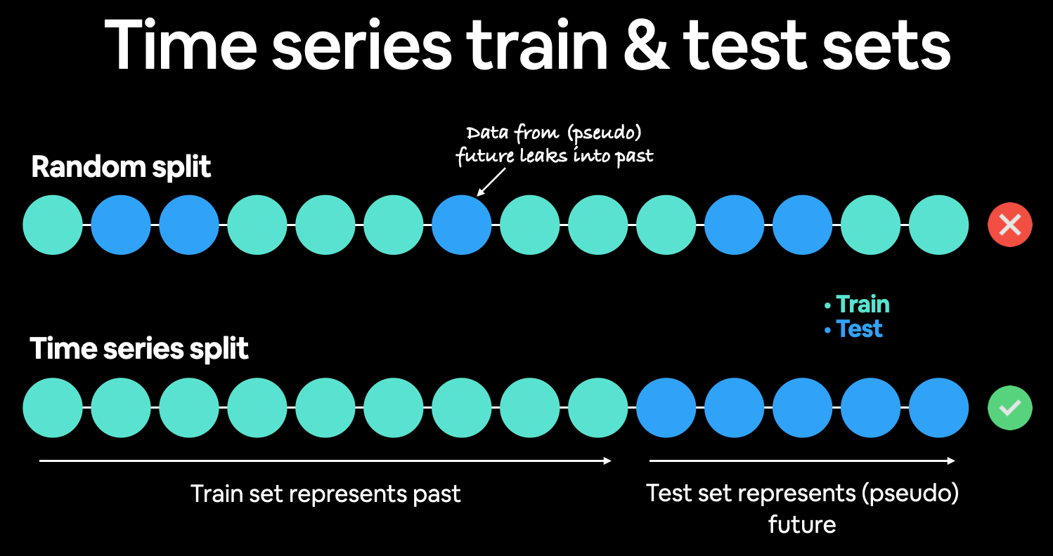
The training and sets are very much overlapping. In real world, the test set for a time series data would be the data that is about to come (in the future). Hence, the above split is wrong, as some test data points are before the training data points, meaning thereby we are using the training data points to predict the past as well.

2. Create train and test sets the right way¶

The right way to create the test set is to emulate how we expect the real world test data to come i.e. the future. So we take train dataset as the past data points (80%), and the test data as the future data points (20%).

In [ ]:

train_prop = 0.8
train_size = int(train_prop * len(prices))
X_train, y_train = timesteps[:train_size], prices[:train_size]
X_test, y_test = timesteps[train_size:], prices[train_size:]

len(X_train), len(X_test)
train_prop = 0.8
train_size = int(train_prop * len(prices))
X_train, y_train = timesteps[:train_size], prices[:train_size]
X_test, y_test = timesteps[train_size:], prices[train_size:]

len(X_train), len(X_test)

Out[ ]:

(2258, 565)

Now let us plot it

In [ ]:

plt.figure(figsize=(12, 7))
plt.scatter(X_train, y_train, label='train', s=5)
plt.scatter(X_test, y_test, label='test', s=5)
plt.xlabel('Date')
plt.ylabel(SELECT_COLUMN);
plt.legend()
plt.title('Splitting time series data into train and test sets (the right way)',
          fontdict=dict(size=15, weight='bold'));
plt.figure(figsize=(12, 7))
plt.scatter(X_train, y_train, label='train', s=5)
plt.scatter(X_test, y_test, label='test', s=5)
plt.xlabel('Date')
plt.ylabel(SELECT_COLUMN);
plt.legend()
plt.title('Splitting time series data into train and test sets (the right way)',
          fontdict=dict(size=15, weight='bold'));

Note: The splits can vary 80/20, 90/10, 95/5 depending upon the amount of data you have. We might even have much data, in which case we can use AIC/BIC or other such model fit metrics.

Resource: The trickier aspects of time series modelling. See: 3 facts about time series forecasting that surprise experienced machine learning practitioners

In [ ]:

def plot_bitcoin(tsteps, prices, linetype='.', start=0, end=None, label=None):

    plt.plot(tsteps[start:end], prices[start:end], linetype, label=label)
    plt.xlabel('Date')
    plt.ylabel(SELECT_COLUMN)
    if label:
        plt.legend(fontsize=15)

    plt.grid(True)
def plot_bitcoin(tsteps, prices, linetype='.', start=0, end=None, label=None):

    plt.plot(tsteps[start:end], prices[start:end], linetype, label=label)
    plt.xlabel('Date')
    plt.ylabel(SELECT_COLUMN)
    if label:
        plt.legend(fontsize=15)

    plt.grid(True)

In [ ]:

plt.figure(figsize=(12, 7))
plot_bitcoin(X_train, y_train, linetype='-', label='Train data')
plot_bitcoin(X_test, y_test, linetype='-', label='Test data')
plt.figure(figsize=(12, 7))
plot_bitcoin(X_train, y_train, linetype='-', label='Train data')
plot_bitcoin(X_test, y_test, linetype='-', label='Test data')

Modelling Experiments¶

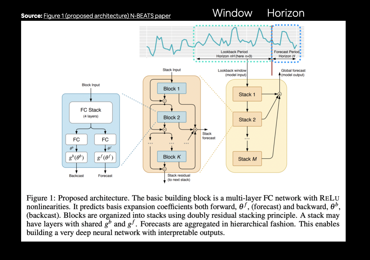
Two terms are really important in the type of forecasting model we are going to build:

Window - The number of timesteps we take to predict into the future
Horizon - The number of timesteps ahead into the future we predict.

For example, a weather forecasting model with Window = 7, and Horizon = 2, uses the last 7 days weather information to predict the next two days' weather.

Model Number	Model Type	Horizon size	Window size	Extra data
0	Naïve forecast model (baseline)	NA	NA	NA
1	Dense model	1	7	NA
2	Dense model variation	1	30	NA
3	Dense model variation	7	30	NA
4	Conv1D	1	7	NA
5	LSTM	1	7	NA
6	Dense model variation (but with multivariate data)	1	7	Block reward size
7	N-BEATs Algorithm	1	7	NA
8	Ensemble (multiple models optimized on different loss functions)	1	7	NA
9	Future prediction model (model to predict future values)	1	7	NA
10	Dense Model variation (but with turkey 🦃 data introduced)	1	7	NA

In [ ]:

MODELS = {}
MODELS_INFO = {}
RESULTS = {}
PREDICTIONS = {}
MODELS = {}
MODELS_INFO = {}
RESULTS = {}
PREDICTIONS = {}

Model 0: Naive Forecast (Baseline)¶

This is the most common baseline model for time series forecasting, which just sets the future one-day ahead forecast as the current day value.

$$\hat{y_t} = y_{t-1}$$

The estimate of the tth timestep is just equal to the value of the t-1th

In [ ]:

WINDOW = 1
HORIZON = 1
WINDOW = 1
HORIZON = 1

In [ ]:

model_name = f'naive-model-baseline_W{WINDOW}H{HORIZON}'
model_name = f'naive-model-baseline_W{WINDOW}H{HORIZON}'

In [ ]:

def naive_model(y):
    return y[:-1]

naive_forecast = naive_model(y_test)
PREDICTIONS[model_name] = naive_forecast
def naive_model(y):
    return y[:-1]

naive_forecast = naive_model(y_test)
PREDICTIONS[model_name] = naive_forecast

In [ ]:

MODELS[model_name] = naive_model
MODELS[model_name] = naive_model

In [ ]:

plt.figure(figsize=(12, 7))
plot_bitcoin(tsteps=X_test, prices=y_test, label='test data')
plot_bitcoin(tsteps=X_test[1:], prices=naive_forecast, linetype='-', label='Naive forecast')
plt.figure(figsize=(12, 7))
plot_bitcoin(tsteps=X_test, prices=y_test, label='test data')
plot_bitcoin(tsteps=X_test[1:], prices=naive_forecast, linetype='-', label='Naive forecast')

Evaluating a time series model¶

Evaluation of a time series can be carried at various levels of n_head forecast horizons. A model trained for any horizon (= 1, say), can be used to forecast to an arbitrary future timesteps ahead by utilising its own predictions in a recursive manner.
For the above model, we can calculate various continous value evaluation metrics such as MAE, RMSE

Scale-dependent errors¶¶

These are metrics which can be used to compare time series values and forecasts that are on the same scale.

For example, Bitcoin historical prices in USD veresus Bitcoin forecast values in USD.

Metric	Details	Code
MAE (mean absolute error)	Easy to interpret (a forecast is X amount different from actual amount). Forecast methods which minimises the MAE will lead to forecasts of the median.	`tf.keras.metrics.mean_absolute_error()`
RMSE (root mean square error)	Forecasts which minimise the RMSE lead to forecasts of the mean.	`tf.sqrt(tf.keras.metrics.mean_square_error())`

Percentage errors¶¶

Percentage errors do not have units, this means they can be used to compare forecasts across different datasets.

Metric	Details	Code
MAPE (mean absolute percentage error)	Most commonly used percentage error. May explode (not work) if `y=0`.	`tf.keras.metrics.mean_absolute_percentage_error()`
sMAPE (scaled mean absolute percentage error)	Recommended not to be used by Forecasting: Principles and Practice, though it is used in forecasting competitions.	Custom implementation

Scaled errors¶¶

Scaled errors are an alternative to percentage errors when comparing forecast performance across different time series.

Metric	Details	Code
MASE (mean absolute scaled error).	MASE equals one for the naive forecast (or very close to one). A forecast which performs better than the naïve should get <1 MASE.	See sktime's `mase_loss()`

In [ ]:

import tensorflow as tf
import tensorflow as tf

In [ ]:

# Compared to the naive forecast, what is my MAE?
def mean_absolute_scaled_error(y_true, y_pred):
    ''' Return MASE (assuming no seasonality in the data)'''
    mae = tf.reduce_mean(tf.abs(y_true - y_pred), axis=1)

    mae_naive_no_seasonlity = tf.reduce_mean(tf.abs(y_true[1:] - y_pred[:-1]), axis=1)

    return mae / mae_naive_no_seasonlity
# Compared to the naive forecast, what is my MAE?
def mean_absolute_scaled_error(y_true, y_pred):
    ''' Return MASE (assuming no seasonality in the data)'''
    mae = tf.reduce_mean(tf.abs(y_true - y_pred), axis=1)

    mae_naive_no_seasonlity = tf.reduce_mean(tf.abs(y_true[1:] - y_pred[:-1]), axis=1)

    return mae / mae_naive_no_seasonlity

For a naive forecast the MASE will be 1. For a model better than the naive forecast, it should be less than 1.
- Worse model: MASE > 1
- Better model: MASE < 1

In [ ]:

from sklearn import metrics as skmetrics
import numpy as np
from sklearn import metrics as skmetrics
import numpy as np

In [ ]:

def evaluate_preds(y_true, y_pred):
    # Make sure the predictions are in float32 format
    y_true = np.broadcast_to(tf.cast(y_true, dtype=tf.float32), y_pred.shape)
    y_pred = tf.cast(y_pred, dtype=tf.float32).numpy()

    # Calculate all the metrics
    mae = skmetrics.mean_absolute_error(y_true, y_pred, multioutput='raw_values')
    mse = skmetrics.mean_squared_error(y_true, y_pred, multioutput='raw_values')
    rmse = np.sqrt(mse)
    mape = skmetrics.mean_absolute_percentage_error(y_true, y_pred, multioutput='raw_values')
    # mase = mean_absolute_scaled_error(y_true, y_pred)

    return {
        'mae': mae,
        'mse': mse,
        'rmse': rmse,
        'mape': mape,
    }
def evaluate_preds(y_true, y_pred):
    # Make sure the predictions are in float32 format
    y_true = np.broadcast_to(tf.cast(y_true, dtype=tf.float32), y_pred.shape)
    y_pred = tf.cast(y_pred, dtype=tf.float32).numpy()

    # Calculate all the metrics
    mae = skmetrics.mean_absolute_error(y_true, y_pred, multioutput='raw_values')
    mse = skmetrics.mean_squared_error(y_true, y_pred, multioutput='raw_values')
    rmse = np.sqrt(mse)
    mape = skmetrics.mean_absolute_percentage_error(y_true, y_pred, multioutput='raw_values')
    # mase = mean_absolute_scaled_error(y_true, y_pred)

    return {
        'mae': mae,
        'mse': mse,
        'rmse': rmse,
        'mape': mape,
    }

In [ ]:

RESULTS[model_name] = evaluate_preds(y_test[1:], naive_forecast)
RESULTS[model_name]
RESULTS[model_name] = evaluate_preds(y_test[1:], naive_forecast)
RESULTS[model_name]

Out[ ]:

{'mae': array([645.9816], dtype=float32),
 'mape': array([0.02631178], dtype=float32),
 'mse': array([1368900.2], dtype=float32),
 'rmse': array([1170.0001], dtype=float32)}

In [ ]:

# Fine the average price of Bitcoin in test dataset
tf.reduce_mean(y_test).numpy()
# Fine the average price of Bitcoin in test dataset
tf.reduce_mean(y_test).numpy()

Out[ ]:

21796.140229169752

We can interpret this as follows:

The average price in our bitcoin dataset is \$20,056 (Since there is one large peak which has its value almost 3x the average), this metric might give a skewed view of the interpretation
Each prediction is off by \$645

Depends on how much close to the true value we want our estimate to be, this might or might not be a good model.

Various time series models which we can use for a baseline estimation¶

Model/Library Name	Resource
Moving average	https://machinelearningmastery.com/moving-average-smoothing-for-time-series-forecasting-python/
ARIMA (Autoregression Integrated Moving Average)	https://machinelearningmastery.com/arima-for-time-series-forecasting-with-python/
sktime (Scikit-Learn for time series)	https://github.com/alan-turing-institute/sktime
TensorFlow Decision Forests (random forest, gradient boosting trees)	https://www.tensorflow.org/decision_forests
Facebook Kats (purpose-built forecasting and time series analysis library by Facebook)	https://github.com/facebookresearch/Kats
LinkedIn Greykite (flexible, intuitive and fast forecasts)	https://github.com/linkedin/greykite

Formatting data - 2. Windowing the dataset¶

Windowing is a method for turning a time series dataset into supervised learning problem
For example, for a model with window=7 and horizon=1, the window-horizon pair will look like:

Data = [0, 1, 2, 3, 4, 5, 6, 7, 8, 9] \

[0, 1, 2, 3, 4, 5, 6] -> [7] \ [1, 2, 3, 4, 5, 6, 7] -> [8] \ [2, 3, 4, 5, 6, 7, 8] -> [9] \

In [ ]:

HORIZON = 1
WINDOW = 7
HORIZON = 1
WINDOW = 7

In [ ]:

def get_labelled_windows(x, horizon=1):
    return x[:, :-horizon], x[:, -horizon:]
def get_labelled_windows(x, horizon=1):
    return x[:, :-horizon], x[:, -horizon:]

In [ ]:

test_window, test_label = get_labelled_windows(tf.expand_dims(tf.range(8) +1, axis=0), horizon=HORIZON)
print(f'Window: {tf.squeeze(test_window).numpy()} -> Label: {tf.squeeze(test_label.numpy())}')
test_window, test_label = get_labelled_windows(tf.expand_dims(tf.range(8) +1, axis=0), horizon=HORIZON)
print(f'Window: {tf.squeeze(test_window).numpy()} -> Label: {tf.squeeze(test_label.numpy())}')

Window: [1 2 3 4 5 6 7] -> Label: 8

In [ ]:

import numpy as np
import numpy as np

In [ ]:

def make_window_horizon_pairs(x, window, horizon):
    window_step = np.expand_dims(np.arange(window + horizon), axis=0)
    window_adders = np.expand_dims(np.arange(len(x) - (window + horizon - 1)), axis=0).T
    window_indices = window_step + window_adders

    windowed_array = x[window_indices]
    windows, labels = get_labelled_windows(windowed_array, horizon)

    return windows, labels
def make_window_horizon_pairs(x, window, horizon):
    window_step = np.expand_dims(np.arange(window + horizon), axis=0)
    window_adders = np.expand_dims(np.arange(len(x) - (window + horizon - 1)), axis=0).T
    window_indices = window_step + window_adders

    windowed_array = x[window_indices]
    windows, labels = get_labelled_windows(windowed_array, horizon)

    return windows, labels

In [ ]:

full_windows, full_labels = make_window_horizon_pairs(prices, window=WINDOW, horizon=HORIZON)
len(full_windows), len(full_labels)
full_windows, full_labels = make_window_horizon_pairs(prices, window=WINDOW, horizon=HORIZON)
len(full_windows), len(full_labels)

Out[ ]:

(2816, 2816)

In [ ]:

# View first three window horizon pairs
for i in range(3):
    print(f'Window: {full_windows[i]} -> Label: {full_labels[i]}')
# View first three window horizon pairs
for i in range(3):
    print(f'Window: {full_windows[i]} -> Label: {full_labels[i]}')

Window: [123.65499 125.455   108.58483 118.67466 121.33866 120.65533 121.795  ] -> Label: [123.033]
Window: [125.455   108.58483 118.67466 121.33866 120.65533 121.795   123.033  ] -> Label: [124.049]
Window: [108.58483 118.67466 121.33866 120.65533 121.795   123.033   124.049  ] -> Label: [125.96116]

Note: The function tf.keras.preprocessing.timeseries_dataset_from_array() does a similar job of preparing the dataset in such a format + has the added advantage of returning a tf.data.Dataset object which offers several benefits over traditional numpy array datasets.

Turning windows into training and test sets¶

In [ ]:

def make_train_test_splits(windows, labels, test_prop=0.2):
    split_size = int(len(windows)*(1-test_prop))
    train_windows, train_labels = windows[:split_size], labels[:split_size]
    test_windows, test_labels = windows[split_size:], labels[split_size:]

    return train_windows, train_labels, test_windows, test_labels
def make_train_test_splits(windows, labels, test_prop=0.2):
    split_size = int(len(windows)*(1-test_prop))
    train_windows, train_labels = windows[:split_size], labels[:split_size]
    test_windows, test_labels = windows[split_size:], labels[split_size:]

    return train_windows, train_labels, test_windows, test_labels

In [ ]:

train_windows, train_labels, test_windows, test_labels = make_train_test_splits(full_windows, full_labels)
len(train_windows), len(test_windows)
train_windows, train_labels, test_windows, test_labels = make_train_test_splits(full_windows, full_labels)
len(train_windows), len(test_windows)

Out[ ]:

(2252, 564)

So now, we have split the time series data into 80%-20% splits.

Make a modelling checkpoint¶

We want to compare each model's best performance against each other. For this reason we would use ModelCheckpoint callback to save the best model weights during training. This would also help us resume training.

In [ ]:

import tensorflow as tf
import tensorflow as tf

In [ ]:

TASK = 'bitcoin_time_series_prediction'
def create_model_checkpoint(model_name):
    return tf.keras.callbacks.ModelCheckpoint(f'../checkpoints/{TASK}/{model_name}', verbose=0, save_best_only=True)
TASK = 'bitcoin_time_series_prediction'
def create_model_checkpoint(model_name):
    return tf.keras.callbacks.ModelCheckpoint(f'../checkpoints/{TASK}/{model_name}', verbose=0, save_best_only=True)

In [ ]:

from src.visualize import plot_learning_curve
from src.visualize import plot_learning_curve

Function for easy training and reloading of `KerasModel`¶

In [ ]:

CHECKPOINT_DIR = f'../checkpoints/bitcoin_time_series_prediction/'
HISTORY_LOG_DIR = f'../history_logs/bitcoin_time_series_prediction/'
CHECKPOINT_DIR = f'../checkpoints/bitcoin_time_series_prediction/'
HISTORY_LOG_DIR = f'../history_logs/bitcoin_time_series_prediction/'

In [ ]:

import json

def train_keras_model(training_func, model_name, 
                      model_or_checkpoint_dir=CHECKPOINT_DIR, history_log_dir=HISTORY_LOG_DIR):
    
    model_or_checkpoint_dir = os.path.join(model_or_checkpoint_dir, model_name)
    history_log_dir = os.path.join(history_log_dir, f'{model_name}.json')

    try:
        model = tf.keras.models.load_model(model_or_checkpoint_dir)
        print('loaded model successfully!')

        with open(history_log_dir, 'r') as f:
            history_dict = json.load(f)

        print('loaded history_dict successfully!')
    
    except Exception:
        history = training_func()
        history_dict = history.history
        model = history.model

        with open(history_log_dir, 'w') as f:
            json.dump(history_dict, f)


    
    return model, history_dict # Because I know the format of return value
import json

def train_keras_model(training_func, model_name, 
                      model_or_checkpoint_dir=CHECKPOINT_DIR, history_log_dir=HISTORY_LOG_DIR):
    
    model_or_checkpoint_dir = os.path.join(model_or_checkpoint_dir, model_name)
    history_log_dir = os.path.join(history_log_dir, f'{model_name}.json')

    try:
        model = tf.keras.models.load_model(model_or_checkpoint_dir)
        print('loaded model successfully!')

        with open(history_log_dir, 'r') as f:
            history_dict = json.load(f)

        print('loaded history_dict successfully!')
    
    except Exception:
        history = training_func()
        history_dict = history.history
        model = history.model

        with open(history_log_dir, 'w') as f:
            json.dump(history_dict, f)


    
    return model, history_dict # Because I know the format of return value

Model 1: Dense Model (Window = 7, Horizon = 1)¶

We will create a simple Dense model which takes in 7 preceding timesteps as input and predicts 1 day ahead.

This will be the configuration of the simple dense model:

A single dense layer with 128 neurons
An output layer with no activation
Adam optimizer and MAE loss function
Batch size of 128
100 epochs

In [ ]:

model_name = 'simple-dense_W7H1'
model_name = 'simple-dense_W7H1'

In [ ]:

from tensorflow.keras import layers

model = tf.keras.Sequential([
    layers.Dense(128, activation='relu', input_shape=(WINDOW,)),
    layers.Dense(HORIZON, activation='linear')
], name=model_name)

model.compile(loss='mae', optimizer=tf.keras.optimizers.Adam(), metrics=['mse'])

model.summary()
from tensorflow.keras import layers

model = tf.keras.Sequential([
    layers.Dense(128, activation='relu', input_shape=(WINDOW,)),
    layers.Dense(HORIZON, activation='linear')
], name=model_name)

model.compile(loss='mae', optimizer=tf.keras.optimizers.Adam(), metrics=['mse'])

model.summary()

Model: "simple-dense_W7H1"
_________________________________________________________________
Layer (type)                 Output Shape              Param #   
=================================================================
dense (Dense)                (None, 128)               1024      
_________________________________________________________________
dense_1 (Dense)              (None, 1)                 129       
=================================================================
Total params: 1,153
Trainable params: 1,153
Non-trainable params: 0
_________________________________________________________________

Training function¶

In [ ]:

def training_func():
     history = model.fit(train_windows, train_labels, 
                validation_data=(test_windows, test_labels), # Ideally these should have been called validation_windows, validation_labels
                epochs=100,
                batch_size=128,
                callbacks=[create_model_checkpoint(model_name=model_name)])
     
     return history
def training_func():
     history = model.fit(train_windows, train_labels, 
                validation_data=(test_windows, test_labels), # Ideally these should have been called validation_windows, validation_labels
                epochs=100,
                batch_size=128,
                callbacks=[create_model_checkpoint(model_name=model_name)])
     
     return history

In [ ]:

model, history_dict = train_keras_model(training_func, model_name)
    
MODELS[model_name] = model
model, history_dict = train_keras_model(training_func, model_name)
    
MODELS[model_name] = model

loaded model successfully!
loaded history_dict successfully!

Since the dataset is so small, the model trains really fast, even in CPU.

Learning curve¶

In [ ]:

plot_learning_curve(history_dict, extra_metric='mse');
plot_learning_curve(history_dict, extra_metric='mse');

Making forecasts with a time series model¶

In [ ]:

def make_preds(model, data):
    return tf.squeeze(model.predict(data))
def make_preds(model, data):
    return tf.squeeze(model.predict(data))

In [ ]:

test_windows.shape
test_windows.shape

Out[ ]:

(564, 7)

In [ ]:

test_labels.shape
test_labels.shape

Out[ ]:

(564, 1)

In [ ]:

preds = make_preds(model, test_windows)
PREDICTIONS[model_name] = preds
preds = make_preds(model, test_windows)
PREDICTIONS[model_name] = preds

In [ ]:

results = evaluate_preds(tf.squeeze(test_labels), preds)
RESULTS[model_name] = results
results
results = evaluate_preds(tf.squeeze(test_labels), preds)
RESULTS[model_name] = results
results

Out[ ]:

{'mae': array([657.3211], dtype=float32),
 'mape': array([0.02734248], dtype=float32),
 'mse': array([1407883.4], dtype=float32),
 'rmse': array([1186.5426], dtype=float32)}

In [ ]:

plt.figure(figsize=(12, 7))
plot_bitcoin(tsteps=X_test[-len(test_windows):], prices=test_labels[:, 0], label='test data')
plot_bitcoin(tsteps=X_test[-len(test_windows):], prices=preds, linetype='-', label='prediction')
plt.figure(figsize=(12, 7))
plot_bitcoin(tsteps=X_test[-len(test_windows):], prices=test_labels[:, 0], label='test data')
plot_bitcoin(tsteps=X_test[-len(test_windows):], prices=preds, linetype='-', label='prediction')

These predictions are not the actual forecasts but predictions on the test dataset for Window = 7 and Horizon = 1

Model 2: Dense (Window = 30, horizon = 1)¶

We will keep the previous model architecture, but make the window size = 30 i.e. we will use the past 30 timesteps to predict the next day.

In [ ]:

HORIZON = 1
WINDOW = 30
HORIZON = 1
WINDOW = 30

Make window-horizon pair dataset¶

In [ ]:

full_windows, full_labels = make_window_horizon_pairs(prices, window=WINDOW, horizon=HORIZON)
full_windows.shape, full_labels.shape
full_windows, full_labels = make_window_horizon_pairs(prices, window=WINDOW, horizon=HORIZON)
full_windows.shape, full_labels.shape

Out[ ]:

((2793, 30), (2793, 1))

Make train test splits¶

In [ ]:

train_windows, train_labels, test_windows, test_labels = make_train_test_splits(full_windows, full_labels)
len(train_windows), len(test_windows)
train_windows, train_labels, test_windows, test_labels = make_train_test_splits(full_windows, full_labels)
len(train_windows), len(test_windows)

Out[ ]:

(2234, 559)

In [ ]:

model_name = f'simple-dense_W{WINDOW}H{HORIZON}'
model_name = f'simple-dense_W{WINDOW}H{HORIZON}'

In [ ]:

tf.random.set_seed(42)

model = tf.keras.Sequential([
    layers.Dense(128, activation='relu', input_shape=(WINDOW,)),
    layers.Dense(HORIZON, activation='linear')
], name=model_name)

model.compile(loss='mae', optimizer=tf.keras.optimizers.Adam(), metrics=['mse'])

model.summary()
tf.random.set_seed(42)

model = tf.keras.Sequential([
    layers.Dense(128, activation='relu', input_shape=(WINDOW,)),
    layers.Dense(HORIZON, activation='linear')
], name=model_name)

model.compile(loss='mae', optimizer=tf.keras.optimizers.Adam(), metrics=['mse'])

model.summary()

Model: "simple-dense_W30H1"
_________________________________________________________________
Layer (type)                 Output Shape              Param #   
=================================================================
dense_2 (Dense)              (None, 128)               3968      
_________________________________________________________________
dense_3 (Dense)              (None, 1)                 129       
=================================================================
Total params: 4,097
Trainable params: 4,097
Non-trainable params: 0
_________________________________________________________________

In [ ]:

def training_func():
    history = model.fit(train_windows, train_labels,
                        validation_data=(test_windows, test_labels), 
                        epochs=100, batch_size=128,
                        callbacks=[create_model_checkpoint(model_name=model_name)])
    
    return history
def training_func():
    history = model.fit(train_windows, train_labels,
                        validation_data=(test_windows, test_labels), 
                        epochs=100, batch_size=128,
                        callbacks=[create_model_checkpoint(model_name=model_name)])
    
    return history

In [ ]:

model, history_dict = train_keras_model(training_func, model_name)    

MODELS[model_name] = model
model, history_dict = train_keras_model(training_func, model_name)    

MODELS[model_name] = model

loaded model successfully!
loaded history_dict successfully!

Learning curve¶

In [ ]:

plot_learning_curve(history_dict, extra_metric='mse');
plot_learning_curve(history_dict, extra_metric='mse');

Get predictions¶

In [ ]:

preds = make_preds(model, test_windows)
PREDICTIONS[model_name] = preds
preds = make_preds(model, test_windows)
PREDICTIONS[model_name] = preds

Evaluate the model¶

In [ ]:

results = evaluate_preds(tf.squeeze(test_labels), preds)
RESULTS[model_name] = results 
results
results = evaluate_preds(tf.squeeze(test_labels), preds)
RESULTS[model_name] = results 
results

Out[ ]:

{'mae': array([695.2544], dtype=float32),
 'mape': array([0.02886072], dtype=float32),
 'mse': array([1513971.9], dtype=float32),
 'rmse': array([1230.4357], dtype=float32)}

In [ ]:

pd.set_option('display.float_format', lambda x: '%.3f'%x)
pd.set_option('display.float_format', lambda x: '%.3f'%x)

In [ ]:

pd.DataFrame(RESULTS)
pd.DataFrame(RESULTS)

Out[ ]:

	naive-model-baseline_W1H1	simple-dense_W7H1	simple-dense_W30H1
mae	[645.9816]	[657.3211]	[695.2544]
mse	[1368900.2]	[1407883.4]	[1513971.9]
rmse	[1170.0001]	[1186.5426]	[1230.4357]
mape	[0.026311785]	[0.027342476]	[0.028860716]

The 30 window model performed worse than the 7 window model!

In [ ]:

plt.figure(figsize=(10, 7))
plot_bitcoin(tsteps=X_test[-len(test_windows):], prices=test_labels[:, 0], label='test data')
plot_bitcoin(tsteps=X_test[-len(test_windows):], prices=test_labels[:, 0], linetype='-', label='predicted')
plt.figure(figsize=(10, 7))
plot_bitcoin(tsteps=X_test[-len(test_windows):], prices=test_labels[:, 0], label='test data')
plot_bitcoin(tsteps=X_test[-len(test_windows):], prices=test_labels[:, 0], linetype='-', label='predicted')

Model 3: Dense (Window = 30, horizon = 7)¶

Now we will predict a week ahead (horizon = 7) using all the past month data (window = 30)

Make window horizon pairs¶

In [ ]:

HORIZON = 7
WINDOW = 30

full_windows, full_labels = make_window_horizon_pairs(prices, window=WINDOW, horizon=HORIZON)
full_windows.shape, full_labels.shape
HORIZON = 7
WINDOW = 30

full_windows, full_labels = make_window_horizon_pairs(prices, window=WINDOW, horizon=HORIZON)
full_windows.shape, full_labels.shape

Out[ ]:

((2787, 30), (2787, 7))

Make train test splits¶

In [ ]:

train_windows, train_labels, test_windows, test_labels = make_train_test_splits(full_windows, full_labels)
len(train_windows), len(test_windows)
train_windows, train_labels, test_windows, test_labels = make_train_test_splits(full_windows, full_labels)
len(train_windows), len(test_windows)

Out[ ]:

(2229, 558)

We will again use the same architechture as model 1

In [ ]:

model_name = f'simple-dense_W{WINDOW}H{HORIZON}'
model_name = f'simple-dense_W{WINDOW}H{HORIZON}'

In [ ]:

model = tf.keras.Sequential([
    layers.Dense(128, activation='relu', input_shape=(WINDOW,)),
    layers.Dense(HORIZON, activation='linear')
], name=model_name)

model.compile(loss='mae', optimizer=tf.keras.optimizers.Adam(), metrics=['mse'])

model.summary()
model = tf.keras.Sequential([
    layers.Dense(128, activation='relu', input_shape=(WINDOW,)),
    layers.Dense(HORIZON, activation='linear')
], name=model_name)

model.compile(loss='mae', optimizer=tf.keras.optimizers.Adam(), metrics=['mse'])

model.summary()

Model: "simple-dense_W30H7"
_________________________________________________________________
Layer (type)                 Output Shape              Param #   
=================================================================
dense_4 (Dense)              (None, 128)               3968      
_________________________________________________________________
dense_5 (Dense)              (None, 7)                 903       
=================================================================
Total params: 4,871
Trainable params: 4,871
Non-trainable params: 0
_________________________________________________________________

In [ ]:

def training_func():
    return model.fit(train_windows, train_labels, validation_data=(test_windows, test_labels),
          batch_size=128, epochs=100, verbose=0,
          callbacks=[create_model_checkpoint(model_name=model_name)])
def training_func():
    return model.fit(train_windows, train_labels, validation_data=(test_windows, test_labels),
          batch_size=128, epochs=100, verbose=0,
          callbacks=[create_model_checkpoint(model_name=model_name)])

In [ ]:

model, history_dict = train_keras_model(training_func, model_name)    

MODELS[model_name] = model
model, history_dict = train_keras_model(training_func, model_name)    

MODELS[model_name] = model

loaded model successfully!
loaded history_dict successfully!

Make predictions¶

In [ ]:

preds = make_preds(model, test_windows)
preds.shape
preds = make_preds(model, test_windows)
preds.shape

Out[ ]:

TensorShape([558, 7])

Evaluate the predictions¶

We have predictions for each time step in the horizon. Hence our error metrics will also be for 7 timesteps in the horizon.

In [ ]:

results = evaluate_preds(tf.broadcast_to(test_labels, preds.shape), preds)
RESULTS[model_name] = results
results
results = evaluate_preds(tf.broadcast_to(test_labels, preds.shape), preds)
RESULTS[model_name] = results
results

Out[ ]:

{'mae': array([ 765.6764,  985.5112, 1252.9808, 1483.6759, 1665.6678, 1832.3729,
        2038.6433], dtype=float32),
 'mape': array([0.03302484, 0.04054034, 0.0505597 , 0.05939244, 0.06612409,
        0.07350221, 0.08160087], dtype=float32),
 'mse': array([ 1736351.6,  3018528. ,  4652685.5,  6375201. ,  8422235. ,
        10376389. , 12933791. ], dtype=float32),
 'rmse': array([1317.7069, 1737.3911, 2157.0085, 2524.916 , 2902.1086, 3221.2402,
        3596.358 ], dtype=float32)}

1-Day ahead forecast¶

In [ ]:

plt.figure(figsize=(12, 7))
plot_bitcoin(tsteps=X_test[-len(test_windows):], prices=test_labels[:, 0], label='test data')
plot_bitcoin(tsteps=X_test[-len(test_windows):], prices=preds[:, 0], linetype='-', label='test data')
plt.title('1-Day ahead forecast', fontdict=dict(weight='bold', size=20))
plt.figure(figsize=(12, 7))
plot_bitcoin(tsteps=X_test[-len(test_windows):], prices=test_labels[:, 0], label='test data')
plot_bitcoin(tsteps=X_test[-len(test_windows):], prices=preds[:, 0], linetype='-', label='test data')
plt.title('1-Day ahead forecast', fontdict=dict(weight='bold', size=20))

Out[ ]:

Text(0.5, 1.0, '1-Day ahead forecast')

2-Day ahead forecast¶

In [ ]:

plt.figure(figsize=(12, 7))
plot_bitcoin(tsteps=X_test[-len(test_windows):], prices=test_labels[:, 0], start=300, label='test data')
plot_bitcoin(tsteps=X_test[-len(test_windows):], prices=preds[:, 1], start=300, linetype='-', label='test data')
plt.title('1-Day ahead forecast', fontdict=dict(weight='bold', size=20))
plt.figure(figsize=(12, 7))
plot_bitcoin(tsteps=X_test[-len(test_windows):], prices=test_labels[:, 0], start=300, label='test data')
plot_bitcoin(tsteps=X_test[-len(test_windows):], prices=preds[:, 1], start=300, linetype='-', label='test data')
plt.title('1-Day ahead forecast', fontdict=dict(weight='bold', size=20))

Out[ ]:

Text(0.5, 1.0, '1-Day ahead forecast')

Which Dense model is performing best?¶

In [ ]:

def _get_day1_pred(x):
    try:
        return x[0]
    except Exception:
        return x
result_df = pd.DataFrame(RESULTS)
result_df.applymap(_get_day1_pred).loc[['mae']].plot(figsize=(12, 7), kind='bar');

def _get_day1_pred(x):
    try:
        return x[0]
    except Exception:
        return x
result_df = pd.DataFrame(RESULTS)
result_df.applymap(_get_day1_pred).loc[['mae']].plot(figsize=(12, 7), kind='bar');

The Simple Dense model with Window = 7 and Horizon = 30 has the highest 1-day ahead mean_absolute_errori.e. it performs the worst out of all.
Still, the naive baseline model has the best i.e lowest mean_absolute_error rate out of all. But remember, you can't really use it to forecast ahead, as all the predictions will be set to the last timestep, which is set to its last and so on. So it will be a flat prediction.
- One of the main reason why naive forecast performs so good is because time series data has autocorrelation i.e. y_t correlates with y_{t-1}

Model 4: Conv1D¶

In [ ]:

HORIZON = 1
WINDOW = 7
HORIZON = 1
WINDOW = 7

Make window horizon pairs¶

In [ ]:

full_windows, full_labels = make_window_horizon_pairs(prices, window=WINDOW, horizon=HORIZON)
full_windows.shape, full_labels.shape
full_windows, full_labels = make_window_horizon_pairs(prices, window=WINDOW, horizon=HORIZON)
full_windows.shape, full_labels.shape

Out[ ]:

((2816, 7), (2816, 1))

Create train test splits¶

In [ ]:

train_windows, train_labels, test_windows, test_labels = make_train_test_splits(full_windows, full_labels)
len(train_windows), len(test_windows)
train_windows, train_labels, test_windows, test_labels = make_train_test_splits(full_windows, full_labels)
len(train_windows), len(test_windows)

Out[ ]:

(2252, 564)

Alright, now our data is windowed as well as split into train and test sets. Are we prepared now to input the data into the CNN model? Not quite. Here is why..

The Conv1D layer in Tensorflow expects the input to be : (batch_size, timesteps, num_features)

So in our case:

batch_size is 32 which we choose and is taken care of
timesteps is the Window which is set to 7
num_features is the number of features = 1 i.e. the time, which is there but not explicitly reflecting in the shape of the data, hence we need to expand the dimension.

Let us create an expand_dim layer for this.

In [ ]:

x = tf.constant(train_windows[0])
expand_dims_layer = layers.Lambda(lambda x: tf.expand_dims(x, axis=-1))
print(f'Original shape: {x.shape}')
print(f'Expanded shape: {expand_dims_layer(x).shape}')
x = tf.constant(train_windows[0])
expand_dims_layer = layers.Lambda(lambda x: tf.expand_dims(x, axis=-1))
print(f'Original shape: {x.shape}')
print(f'Expanded shape: {expand_dims_layer(x).shape}')

Original shape: (7,)
Expanded shape: (7, 1)

Create the model¶

In [ ]:

model_name = f'Conv1D_W{WINDOW}H{HORIZON}'
model_name = f'Conv1D_W{WINDOW}H{HORIZON}'

In [ ]:

model = tf.keras.Sequential([
    layers.InputLayer(input_shape=(WINDOW,)),
    expand_dims_layer,
    layers.Conv1D(filters=128, kernel_size=5, padding='causal', activation='relu'),
    layers.Flatten(),
    layers.Dense(HORIZON)
], name=model_name)

model.compile(loss='mae', optimizer=tf.keras.optimizers.Adam(), metrics=['mse'])

model.summary()
model = tf.keras.Sequential([
    layers.InputLayer(input_shape=(WINDOW,)),
    expand_dims_layer,
    layers.Conv1D(filters=128, kernel_size=5, padding='causal', activation='relu'),
    layers.Flatten(),
    layers.Dense(HORIZON)
], name=model_name)

model.compile(loss='mae', optimizer=tf.keras.optimizers.Adam(), metrics=['mse'])

model.summary()

Model: "Conv1D_W7H1"
_________________________________________________________________
Layer (type)                 Output Shape              Param #   
=================================================================
lambda (Lambda)              (None, 7, 1)              0         
_________________________________________________________________
conv1d (Conv1D)              (None, 7, 128)            768       
_________________________________________________________________
flatten (Flatten)            (None, 896)               0         
_________________________________________________________________
dense_6 (Dense)              (None, 1)                 897       
=================================================================
Total params: 1,665
Trainable params: 1,665
Non-trainable params: 0
_________________________________________________________________

In [ ]:

def training_func():
    return model.fit(train_windows, train_labels, validation_data=(test_windows, test_labels),
          batch_size=128, epochs=100, callbacks=[create_model_checkpoint(model_name=model_name)])
def training_func():
    return model.fit(train_windows, train_labels, validation_data=(test_windows, test_labels),
          batch_size=128, epochs=100, callbacks=[create_model_checkpoint(model_name=model_name)])

In [ ]:

model, history_dict = train_keras_model(training_func, model_name)    

MODELS[model_name] = model
model, history_dict = train_keras_model(training_func, model_name)    

MODELS[model_name] = model

loaded model successfully!
loaded history_dict successfully!

Learning Curve¶

In [ ]:

plot_learning_curve(history_dict);
plot_learning_curve(history_dict);

Highly, highly overfitted!

Make predictions¶

In [ ]:

preds = make_preds(model, test_windows)
PREDICTIONS[model_name] = preds
preds
preds = make_preds(model, test_windows)
PREDICTIONS[model_name] = preds
preds

Out[ ]:

<tf.Tensor: shape=(564,), dtype=float32, numpy=
array([ 7541.4507,  7538.419 ,  7369.965 ,  7237.2026,  7184.724 ,
        7187.412 ,  7223.9355,  7114.046 ,  7084.255 ,  6921.393 ,
        6631.929 ,  7186.379 ,  7276.2285,  7163.8823,  7198.8374,
        7248.9175,  7206.078 ,  7187.368 ,  7214.822 ,  7191.6914,
        7201.186 ,  7285.3677,  7373.8467,  7282.6475,  7175.0635,
        7152.6455,  7003.6787,  7191.7744,  7337.9785,  7364.6484,
        7612.7056,  7979.748 ,  8113.6357,  7875.896 ,  7981.4604,
        8091.0244,  8157.432 ,  8111.8335,  8574.723 ,  8873.057 ,
        8779.799 ,  8846.266 ,  8930.719 ,  8732.35  ,  8607.697 ,
        8668.239 ,  8669.643 ,  8429.824 ,  8387.077 ,  8361.985 ,
        8510.619 ,  8810.689 ,  9100.28  ,  9304.295 ,  9503.933 ,
        9445.041 ,  9359.061 ,  9356.293 ,  9298.008 ,  9188.378 ,
        9492.299 ,  9700.635 ,  9790.46  ,  9883.514 , 10085.147 ,
        9929.859 , 10114.081 , 10340.126 , 10287.595 , 10307.725 ,
       10007.113 ,  9859.378 ,  9656.468 , 10041.84  ,  9855.681 ,
        9610.647 ,  9598.509 ,  9686.635 ,  9883.508 ,  9699.7705,
        9420.492 ,  8874.922 ,  8719.231 ,  8766.307 ,  8683.228 ,
        8544.305 ,  8793.549 ,  8849.852 ,  8764.271 ,  8967.116 ,
        9133.852 ,  8996.733 ,  8304.699 ,  7863.1914,  7879.417 ,
        7980.547 ,  6333.364 ,  5519.192 ,  5242.038 ,  5365.313 ,
        5047.3066,  5287.1494,  5410.579 ,  6084.9463,  6253.743 ,
        6222.9976,  5943.9224,  6291.8306,  6770.8853,  6788.26  ,
        6710.742 ,  6665.292 ,  6339.411 ,  5959.5957,  6294.047 ,
        6509.752 ,  6548.7217,  6748.091 ,  6810.837 ,  6854.688 ,
        6801.7354,  7163.369 ,  7242.215 ,  7330.912 ,  7325.197 ,
        6970.078 ,  6827.244 ,  6975.6484,  6962.3354,  6874.709 ,
        6720.8228,  7046.123 ,  7122.7676,  7233.6885,  7200.423 ,
        6924.5923,  6855.8154,  7051.611 ,  7497.005 ,  7556.7773,
        7529.1836,  7585.683 ,  7747.339 ,  7787.009 ,  8530.646 ,
        8852.533 ,  8889.89  ,  8918.209 ,  8918.396 ,  8905.227 ,
        8937.319 ,  9283.38  ,  9813.696 ,  9969.903 ,  9701.797 ,
        8936.364 ,  8563.64  ,  8724.303 ,  9254.482 ,  9713.696 ,
        9483.283 ,  9367.356 ,  9585.998 ,  9760.102 ,  9739.926 ,
        9551.698 ,  9204.241 ,  9133.665 ,  9202.079 ,  9102.982 ,
        8908.516 ,  8806.854 ,  9036.312 ,  9438.19  ,  9484.705 ,
        9619.711 ,  9482.682 , 10061.312 ,  9750.354 ,  9602.463 ,
        9720.47  ,  9724.098 ,  9680.5   ,  9675.544 ,  9786.042 ,
        9788.949 ,  9837.089 ,  9398.01  ,  9355.39  ,  9440.887 ,
        9402.332 ,  9398.074 ,  9467.065 ,  9481.166 ,  9395.695 ,
        9281.652 ,  9317.174 ,  9300.972 ,  9581.144 ,  9645.531 ,
        9381.216 ,  9214.246 ,  9158.783 ,  9064.132 ,  9058.662 ,
        9153.888 ,  9164.439 ,  9200.016 ,  9116.636 ,  9079.3955,
        9100.436 ,  9068.736 ,  9215.672 ,  9254.261 ,  9417.577 ,
        9292.253 ,  9219.013 ,  9209.201 ,  9270.924 ,  9253.142 ,
        9235.816 ,  9209.796 ,  9139.027 ,  9135.913 ,  9162.723 ,
        9184.195 ,  9165.945 ,  9328.718 ,  9509.221 ,  9611.161 ,
        9578.073 ,  9659.367 ,  9886.473 , 10920.689 , 11117.455 ,
       11240.623 , 11142.498 , 11313.994 , 11701.682 , 11319.678 ,
       11185.884 , 11180.248 , 11579.72  , 11801.186 , 11679.086 ,
       11691.686 , 11668.261 , 11799.029 , 11453.717 , 11446.039 ,
       11688.332 , 11810.38  , 11867.688 , 11871.409 , 12277.097 ,
       12184.1455, 11808.047 , 11740.367 , 11632.802 , 11654.115 ,
       11641.29  , 11716.611 , 11456.929 , 11387.672 , 11317.536 ,
       11432.908 , 11506.293 , 11616.4375, 11670.207 , 11885.209 ,
       11566.882 , 10829.965 , 10495.851 , 10125.296 , 10149.144 ,
       10321.08  , 10136.389 , 10171.461 , 10293.698 , 10396.121 ,
       10416.16  , 10321.857 , 10578.838 , 10811.986 , 11011.717 ,
       10965.449 , 10915.205 , 11005.288 , 10903.886 , 10583.1875,
       10470.812 , 10306.683 , 10561.194 , 10727.828 , 10752.0625,
       10727.887 , 10814.707 , 10796.883 , 10731.072 , 10629.982 ,
       10561.65  , 10541.093 , 10623.125 , 10734.497 , 10626.674 ,
       10602.295 , 10820.072 , 11041.059 , 11304.902 , 11351.824 ,
       11587.145 , 11507.463 , 11394.204 , 11445.915 , 11392.298 ,
       11350.012 , 11414.252 , 11708.442 , 11924.427 , 12838.35  ,
       13227.715 , 13044.728 , 12996.316 , 13009.268 , 13056.212 ,
       13542.195 , 13432.408 , 13408.624 , 13501.606 , 13834.5205,
       13804.771 , 13623.514 , 13746.213 , 14094.468 , 15171.939 ,
       15624.715 , 15023.148 , 15226.63  , 15336.139 , 15420.499 ,
       15674.178 , 16161.474 , 16391.78  , 16071.379 , 15876.004 ,
       16520.6   , 17485.62  , 17891.977 , 17950.715 , 18437.865 ,
       18653.504 , 18653.883 , 18472.152 , 18876.436 , 18860.46  ,
       17532.754 , 16887.86  , 17518.027 , 18184.225 , 19143.953 ,
       19120.512 , 19143.867 , 19355.191 , 18988.797 , 18953.152 ,
       19043.594 , 19138.79  , 18763.326 , 18487.143 , 18357.648 ,
       18167.207 , 18669.91  , 19054.184 , 19243.746 , 19376.053 ,
       20866.787 , 22661.082 , 23214.098 , 23747.691 , 23681.602 ,
       23295.291 , 23307.537 , 23264.996 , 23543.523 , 24339.664 ,
       26039.207 , 26578.246 , 26698.455 , 26880.615 , 28378.078 ,
       29224.055 , 29382.15  , 31464.473 , 33033.61  , 32064.059 ,
       33544.68  , 35957.75  , 39181.25  , 40475.383 , 40552.406 ,
       39166.594 , 35279.008 , 33885.63  , 36160.625 , 38516.574 ,
       37395.1   , 35880.98  , 36032.992 , 36459.37  , 36586.58  ,
       35280.08  , 31475.176 , 32207.078 , 32447.938 , 32412.895 ,
       32254.977 , 32256.316 , 30995.361 , 32479.887 , 34683.004 ,
       35003.863 , 33398.773 , 33212.48  , 35179.527 , 37280.684 ,
       37506.32  , 37676.35  , 39691.418 , 39154.89  , 43202.21  ,
       46325.125 , 46146.38  , 46919.914 , 47854.812 , 47512.81  ,
       48524.88  , 48381.45  , 48723.805 , 51284.734 , 52128.38  ,
       54924.555 , 55183.75  , 56702.62  , 54947.613 , 49416.992 ,
       47976.594 , 48124.273 , 46627.68  , 46081.348 , 45206.684 ,
       48267.203 , 48453.85  , 50139.547 , 48904.758 , 48797.68  ,
       48847.254 , 50209.16  , 51456.664 , 53803.785 , 56587.883 ,
       57786.133 , 57513.473 , 59832.324 , 60590.742 , 57368.785 ,
       56041.695 , 57880.297 , 58544.902 , 58304.68  , 58310.992 ,
       57961.39  , 55038.566 , 54234.633 , 53143.727 , 52259.53  ,
       53727.582 , 55937.477 , 55828.508 , 56921.89  , 58482.844 ,
       58969.355 , 58906.6   , 58738.94  , 57797.094 , 57851.277 ,
       58635.87  , 58317.816 , 56717.52  , 57241.008 , 58159.215 ,
       59150.22  , 59675.15  , 59821.586 , 62395.65  , 63224.28  ,
       63373.188 , 62152.445 , 60709.473 , 57533.613 , 55949.484 ,
       56332.777 , 54803.555 , 52205.19  , 50473.22  , 50540.72  ,
       49079.32  , 52139.016 , 55018.727 , 55109.867 , 53440.16  ,
       56035.332 , 57992.34  , 57001.152 , 56779.117 , 54358.098 ,
       56231.7   , 56845.254 , 57128.453 , 58244.49  , 58274.3   ,
       56315.215 , 55979.496 , 53115.375 , 50083.406 , 49446.57  ,
       48362.41  , 46060.49  , 43274.54  , 42795.914 , 40290.367 ,
       39354.453 , 37356.01  , 37162.293 , 34919.887 , 36893.395 ,
       38433.51  , 38975.24  , 38707.758 , 35654.906 , 34360.273 ,
       35196.938 , 36908.902 , 36713.86  , 37013.395 , 38566.18  ,
       37801.68  , 35384.46  , 34863.027 , 34309.74  , 33639.746 ,
       36094.535 , 37077.523 , 37340.305 , 35915.684 , 37968.64  ,
       40134.31  , 40465.836 , 38909.88  , 37630.83  , 35908.43  ,
       35460.816 , 35610.227 , 32616.32  , 31842.602 ], dtype=float32)>

Evaluate predictions¶

In [ ]:

preds.shape
preds.shape

Out[ ]:

TensorShape([564])

In [ ]:

test_labels.shape
test_labels.shape

Out[ ]:

(564, 1)

In [ ]:

results = evaluate_preds(tf.squeeze(test_labels), preds)
RESULTS[model_name] = results
results
results = evaluate_preds(tf.squeeze(test_labels), preds)
RESULTS[model_name] = results
results

Out[ ]:

{'mae': array([658.0913], dtype=float32),
 'mape': array([0.02705742], dtype=float32),
 'mse': array([1412351.2], dtype=float32),
 'rmse': array([1188.4238], dtype=float32)}

Did our CNN model work well?¶

In [ ]:

result_df = pd.DataFrame(RESULTS)
result_df.applymap(_get_day1_pred).loc[['mae']].plot(figsize=(12, 7), kind='bar');
result_df = pd.DataFrame(RESULTS)
result_df.applymap(_get_day1_pred).loc[['mae']].plot(figsize=(12, 7), kind='bar');

Not really an improvement :(

Model 5: LSTM¶

LSTM layer in keras also expects the input tensor to be of the shape [batch, timesteps, num_features]

In [ ]:

WINDOW = 7
HORIZON = 1
WINDOW = 7
HORIZON = 1

In [ ]:

model_name = f'LSTM_W{WINDOW}H{HORIZON}'
model_name = f'LSTM_W{WINDOW}H{HORIZON}'

In [ ]:

tf.random.set_seed(42)

model = tf.keras.Sequential([
    layers.InputLayer(input_shape=(WINDOW,)),
    expand_dims_layer,
    layers.LSTM(128, activation='relu'),
    layers.Dense(HORIZON)
], name=model_name)

model.compile(loss='mae', optimizer=tf.keras.optimizers.Adam(), metrics=['mse'])

model.summary()
tf.random.set_seed(42)

model = tf.keras.Sequential([
    layers.InputLayer(input_shape=(WINDOW,)),
    expand_dims_layer,
    layers.LSTM(128, activation='relu'),
    layers.Dense(HORIZON)
], name=model_name)

model.compile(loss='mae', optimizer=tf.keras.optimizers.Adam(), metrics=['mse'])

model.summary()

WARNING:tensorflow:Layer lstm will not use cuDNN kernels since it doesn't meet the criteria. It will use a generic GPU kernel as fallback when running on GPU.
Model: "LSTM_W7H1"
_________________________________________________________________
Layer (type)                 Output Shape              Param #   
=================================================================
lambda (Lambda)              (None, 7, 1)              0         
_________________________________________________________________
lstm (LSTM)                  (None, 128)               66560     
_________________________________________________________________
dense_7 (Dense)              (None, 1)                 129       
=================================================================
Total params: 66,689
Trainable params: 66,689
Non-trainable params: 0
_________________________________________________________________

In [ ]:

def training_func():
    return model.fit(train_windows, train_labels, validation_data=(test_windows, test_labels),
          batch_size=128, epochs=100, callbacks=[create_model_checkpoint(model_name)])
def training_func():
    return model.fit(train_windows, train_labels, validation_data=(test_windows, test_labels),
          batch_size=128, epochs=100, callbacks=[create_model_checkpoint(model_name)])

In [ ]:

model, history_dict = train_keras_model(training_func, model_name)    

MODELS[model_name] = model
model, history_dict = train_keras_model(training_func, model_name)    

MODELS[model_name] = model

WARNING:tensorflow:Layer lstm will not use cuDNN kernels since it doesn't meet the criteria. It will use a generic GPU kernel as fallback when running on GPU.
loaded model successfully!
loaded history_dict successfully!

Make predictions¶

In [ ]:

preds = make_preds(model, test_windows)
preds.shape
preds = make_preds(model, test_windows)
preds.shape

Out[ ]:

TensorShape([564])

Evaluate predictions¶

In [ ]:

results = evaluate_preds(tf.squeeze(test_labels), preds)
RESULTS[model_name] = results
results
results = evaluate_preds(tf.squeeze(test_labels), preds)
RESULTS[model_name] = results
results

Out[ ]:

{'mae': array([763.69543], dtype=float32),
 'mape': array([0.03152551], dtype=float32),
 'mse': array([1799688.5], dtype=float32),
 'rmse': array([1341.5247], dtype=float32)}

Nope, just blindly using LSTM did not improve our result, even over the baseline naive forecast model.

Multivariate time series prediction¶

Till now all of the models could not even beat the baseline naive forecast model which just uses the previous timestep as the next timestep forecast.

Maybe giving the model a bit more information than just the time will help explain the variation in bitcoin prices.

Almost everything, for e.g. tweets, financial news, world news could help increase the predictive power of bitcoin time series forecasting model. It is just upto us, as to how we feed this information to the model.

Here, for now, we will include one more variable, called the Bitcoin block reward size. It is the number of bitcoins one receives from mining a Bitcoin block.

Initially the bitcoin block reward size was 50. But every 4 years approx. the reward size is halved.

In [ ]:

bitcoin_prices.head()
bitcoin_prices.head()

Out[ ]:

	price
date
2013-10-01	123.655
2013-10-02	125.455
2013-10-03	108.585
2013-10-04	118.675
2013-10-05	121.339

Bitcoin block reward and start dates of introduction:

Block Reward	Start Date
50	3 January 2009 (2009-01-03)
25	28 November 2012
12.5	9 July 2016
6.25	11 May 2020
3.125	TBA (expected 2024)
1.5625	TBA (expected 2028)

In [ ]:

bitcoin_price_block_df = bitcoin_prices.copy()
bitcoin_price_block_df['block_reward'] = np.nan
bitcoin_price_block_df
bitcoin_price_block_df = bitcoin_prices.copy()
bitcoin_price_block_df['block_reward'] = np.nan
bitcoin_price_block_df

Out[ ]:

	price	block_reward
date
2013-10-01	123.655	nan
2013-10-02	125.455	nan
2013-10-03	108.585	nan
2013-10-04	118.675	nan
2013-10-05	121.339	nan
...	...	...
2021-06-20	35656.305	nan
2021-06-21	35681.134	nan
2021-06-22	31659.542	nan
2021-06-23	32404.330	nan
2021-06-24	33532.258	nan

2823 rows × 2 columns

In [ ]:

bitcoin_price_block_df.loc['28 November 2012': '9 July 2016', 'block_reward'] = 25
bitcoin_price_block_df.loc['9 July 2016': '11 May 2020', 'block_reward'] = 12.5
bitcoin_price_block_df.loc['11 May 2020':, 'block_reward'] = 6.125
bitcoin_price_block_df.loc['28 November 2012': '9 July 2016', 'block_reward'] = 25
bitcoin_price_block_df.loc['9 July 2016': '11 May 2020', 'block_reward'] = 12.5
bitcoin_price_block_df.loc['11 May 2020':, 'block_reward'] = 6.125

In [ ]:

bitcoin_price_block_df
bitcoin_price_block_df

Out[ ]:

	price	block_reward
date
2013-10-01	123.655	25.000
2013-10-02	125.455	25.000
2013-10-03	108.585	25.000
2013-10-04	118.675	25.000
2013-10-05	121.339	25.000
...	...	...
2021-06-20	35656.305	6.125
2021-06-21	35681.134	6.125
2021-06-22	31659.542	6.125
2021-06-23	32404.330	6.125
2021-06-24	33532.258	6.125

2823 rows × 2 columns

In [ ]:

from sklearn.preprocessing import minmax_scale
bitcoin_price_block_scaled_df = pd.DataFrame(minmax_scale(bitcoin_price_block_df),
                                             columns=bitcoin_price_block_df.columns,
                                             index=bitcoin_price_block_df.index)
bitcoin_price_block_scaled_df.plot(figsize=(12, 7))
from sklearn.preprocessing import minmax_scale
bitcoin_price_block_scaled_df = pd.DataFrame(minmax_scale(bitcoin_price_block_df),
                                             columns=bitcoin_price_block_df.columns,
                                             index=bitcoin_price_block_df.index)
bitcoin_price_block_scaled_df.plot(figsize=(12, 7))

Out[ ]:

<matplotlib.axes._subplots.AxesSubplot at 0x7f7fed0a5f10>

Make a windowed dataset for multivariate data¶

In [ ]:

HORIZON = 1
WINDOW = 7
HORIZON = 1
WINDOW = 7

In [ ]:

bitcoin_prices_windowed = bitcoin_price_block_df.copy()

for i in range(WINDOW):
    bitcoin_prices_windowed[f'price_lag{i+1}'] = bitcoin_prices_windowed['price'].shift(periods=i+1)

bitcoin_prices_windowed.head()
bitcoin_prices_windowed = bitcoin_price_block_df.copy()

for i in range(WINDOW):
    bitcoin_prices_windowed[f'price_lag{i+1}'] = bitcoin_prices_windowed['price'].shift(periods=i+1)

bitcoin_prices_windowed.head()

Out[ ]:

	price	block_reward	price_lag1	price_lag2	price_lag3	price_lag4	price_lag5	price_lag6	price_lag7
date
2013-10-01	123.655	25.000	nan	nan	nan	nan	nan	nan	nan
2013-10-02	125.455	25.000	123.655	nan	nan	nan	nan	nan	nan
2013-10-03	108.585	25.000	125.455	123.655	nan	nan	nan	nan	nan
2013-10-04	118.675	25.000	108.585	125.455	123.655	nan	nan	nan	nan
2013-10-05	121.339	25.000	118.675	108.585	125.455	123.655	nan	nan	nan

In [ ]:

bitcoin_prices_windowed.columns
bitcoin_prices_windowed.columns

Out[ ]:

Index(['price', 'block_reward', 'price_lag1', 'price_lag2', 'price_lag3',
       'price_lag4', 'price_lag5', 'price_lag6', 'price_lag7'],
      dtype='object')

The multivariate model we are going to train will be a Dense model which doesn't really care about the ordering of the sequence

So we can pass the features as

['block_reward', 'price_lag1', 'price_lag2', 'price_lag3', 'price_lag4', 'price_lag5', 'price_lag6', 'price_lag7']

Let us make the $X$ and $y$ for the same

In [ ]:

X = bitcoin_prices_windowed.dropna().drop('price', axis=1).astype(np.float32)
y = bitcoin_prices_windowed.dropna()['price'].astype(np.float32)
X.head()
X = bitcoin_prices_windowed.dropna().drop('price', axis=1).astype(np.float32)
y = bitcoin_prices_windowed.dropna()['price'].astype(np.float32)
X.head()

Out[ ]:

	block_reward	price_lag1	price_lag2	price_lag3	price_lag4	price_lag5	price_lag6	price_lag7
date
2013-10-08	25.000	121.795	120.655	121.339	118.675	108.585	125.455	123.655
2013-10-09	25.000	123.033	121.795	120.655	121.339	118.675	108.585	125.455
2013-10-10	25.000	124.049	123.033	121.795	120.655	121.339	118.675	108.585
2013-10-11	25.000	125.961	124.049	123.033	121.795	120.655	121.339	118.675
2013-10-12	25.000	125.280	125.961	124.049	123.033	121.795	120.655	121.339

In [ ]:

X.shape
X.shape

Out[ ]:

(2816, 8)

SO we have 1 + 7 features i.e. past 7 days bitcoin prices + the block_reward

In [ ]:

y.head()
y.head()

Out[ ]:

date
2013-10-08   123.033
2013-10-09   124.049
2013-10-10   125.961
2013-10-11   125.280
2013-10-12   125.927
Name: price, dtype: float32

Now let us make the train, test splits

In [ ]:

train_prop = 0.8
train_size = int(len(X)*train_prop)
X_train, y_train = X[:train_size], y[:train_size]
X_test, y_test = X[train_size:], y[train_size:]

len(X_train), len(X_test)
train_prop = 0.8
train_size = int(len(X)*train_prop)
X_train, y_train = X[:train_size], y[:train_size]
X_test, y_test = X[train_size:], y[train_size:]

len(X_train), len(X_test)

Out[ ]:

(2252, 564)

Model 6: Dense (multivariate time series)¶

In [ ]:

model_name = f'multivariate-dense_W{WINDOW}H{HORIZON}'
model_name = f'multivariate-dense_W{WINDOW}H{HORIZON}'

In [ ]:

tf.random.set_seed(42)

model = tf.keras.Sequential([
    layers.Dense(128, activation='relu', input_shape=(X_train.shape[1],)),
    layers.Dense(HORIZON)
], name=model_name)

model.compile(loss='mae', optimizer=tf.keras.optimizers.Adam(), metrics=['mse'])

model.summary()
tf.random.set_seed(42)

model = tf.keras.Sequential([
    layers.Dense(128, activation='relu', input_shape=(X_train.shape[1],)),
    layers.Dense(HORIZON)
], name=model_name)

model.compile(loss='mae', optimizer=tf.keras.optimizers.Adam(), metrics=['mse'])

model.summary()

Model: "multivariate-dense_W7H1"
_________________________________________________________________
Layer (type)                 Output Shape              Param #   
=================================================================
dense_8 (Dense)              (None, 128)               1152      
_________________________________________________________________
dense_9 (Dense)              (None, 1)                 129       
=================================================================
Total params: 1,281
Trainable params: 1,281
Non-trainable params: 0
_________________________________________________________________

There is a better way in which we can feed the block_reward size to the model. Since there is a definite order to past 7 days bitcoin prices it must be processed by a sequence model (or using transformer models as well which encode the position without the need to sequentially process them -> hence can process a sequence in parallel!)

For the block reward size, we can learn an embedding i.e. a numerical representation which we can then concatenate with the representation of the sequence data i.e. prices and make our architecture.

In [ ]:

def training_func():

    return model.fit(X_train, y_train, validation_data=(X_test, y_test),
                     batch_size=128, epochs=100, callbacks=[create_model_checkpoint(model_name)])
def training_func():

    return model.fit(X_train, y_train, validation_data=(X_test, y_test),
                     batch_size=128, epochs=100, callbacks=[create_model_checkpoint(model_name)])
    

In [ ]:

model, history_dict = train_keras_model(training_func, model_name)

MODELS[model_name] = model
model, history_dict = train_keras_model(training_func, model_name)

MODELS[model_name] = model

loaded model successfully!
loaded history_dict successfully!

Learning Curve¶

In [ ]:

plot_learning_curve(history_dict, extra_metric='mse');
plot_learning_curve(history_dict, extra_metric='mse');

Make predictions¶

In [ ]:

preds = make_preds(model, X_test)
preds.shape
preds = make_preds(model, X_test)
preds.shape

Out[ ]:

TensorShape([564])

Evaluate predictions¶

In [ ]:

results = evaluate_preds(y_test, preds)
RESULTS[model_name] = results
results
results = evaluate_preds(y_test, preds)
RESULTS[model_name] = results
results

Out[ ]:

{'mae': array([651.629], dtype=float32),
 'mape': array([0.02681939], dtype=float32),
 'mse': array([1388462.9], dtype=float32),
 'rmse': array([1178.3306], dtype=float32)}

Comparing model performance¶

In [ ]:

result_df = pd.DataFrame(RESULTS)
result_df.applymap(_get_day1_pred).loc[['mae']].plot(figsize=(14, 7), kind='bar');
result_df = pd.DataFrame(RESULTS)
result_df.applymap(_get_day1_pred).loc[['mae']].plot(figsize=(14, 7), kind='bar');

Model 7: N-BEATS Algorithm¶

So far we have only tried smaller models. Now we will reimplement the architechture from the paper N-BEATS (Neural Basis Expansion Analysis for Interpretable Time Series Forecasting) algorithm

The N-BEATS model was trained on a univariate time series prediction task and achieved SOTA winning performance on the M4 competition (Kaggle).

Replicating the model architechture

Hyperparameters are listed in Appendix D of the N-BEATS paper

To replicate the above architechture, we will:

Create a custom layer for the NBeatsBlock by subclassing tf.keras.layers.Layer
Implement the full architechture using the Keras functional API

Building the N-BEATS block layer¶

In [ ]:

class NBeatsBlock(tf.keras.layers.Layer):

    def __init__(self,
                 input_size: int,
                 theta_size: int,
                 horizon: int,
                 n_neurons: int,
                 n_layers: int,
                 **kwargs):
        super().__init__(**kwargs)
        self.input_size = input_size
        self.theta_size = theta_size
        self.horizon = horizon
        self.n_neurons = n_neurons
        self.n_layers = n_layers

        self.hidden = [tf.keras.layers.Dense(n_neurons, activation='relu') for _ in range(n_layers)]
        self.theta_layer = tf.keras.layers.Dense(theta_size, activation='linear', name='theta')


    def call(self, inputs):
        x = inputs
        for layer in self.hidden:
            x = layer(x)

        theta = self.theta_layer(x)
        backcast, forecast = theta[:, :self.input_size], theta[:, -self.horizon:]

        return backcast, forecast


    def get_config(self):

        attrs = ['input_size', 'theta_size', 'horizon', 'n_neurons', 'n_layers']
        config = {attr: self.__getattribute__(attr) for attr in attrs}

        return config
class NBeatsBlock(tf.keras.layers.Layer):

    def __init__(self,
                 input_size: int,
                 theta_size: int,
                 horizon: int,
                 n_neurons: int,
                 n_layers: int,
                 **kwargs):
        super().__init__(**kwargs)
        self.input_size = input_size
        self.theta_size = theta_size
        self.horizon = horizon
        self.n_neurons = n_neurons
        self.n_layers = n_layers

        self.hidden = [tf.keras.layers.Dense(n_neurons, activation='relu') for _ in range(n_layers)]
        self.theta_layer = tf.keras.layers.Dense(theta_size, activation='linear', name='theta')


    def call(self, inputs):
        x = inputs
        for layer in self.hidden:
            x = layer(x)

        theta = self.theta_layer(x)
        backcast, forecast = theta[:, :self.input_size], theta[:, -self.horizon:]

        return backcast, forecast


    def get_config(self):

        attrs = ['input_size', 'theta_size', 'horizon', 'n_neurons', 'n_layers']
        config = {attr: self.__getattribute__(attr) for attr in attrs}

        return config

In [ ]:

class NBeatsStack(tf.keras.layers.Layer):

    def __init__(self, block, n_blocks, **kwargs):
        super().__init__(**kwargs)
        self.block = block
        self.block_config = block.get_config()
        self.n_blocks = n_blocks

    def call(self, inputs):
        block_config = {**self.block_config, 'name': f'{self.name}_block0'}
        initial_block = NBeatsBlock.from_config(block_config)
        stack_residuals, stack_forecast = initial_block(inputs)

        for block_num in range(1, self.n_blocks):
            block_config = {**self.block_config, 'name': f'{self.name}_block{block_num}'}
            block = NBeatsBlock.from_config(block_config)
            block_backcast, block_forecast = block(stack_residuals)

            stack_residuals = layers.subtract([stack_residuals, block_backcast], name=f'{block.name}_subtract')
            stack_forecast = layers.add([stack_forecast, block_forecast], name=f'{block.name}_add')

        return stack_residuals, stack_forecast
class NBeatsStack(tf.keras.layers.Layer):

    def __init__(self, block, n_blocks, **kwargs):
        super().__init__(**kwargs)
        self.block = block
        self.block_config = block.get_config()
        self.n_blocks = n_blocks

    def call(self, inputs):
        block_config = {**self.block_config, 'name': f'{self.name}_block0'}
        initial_block = NBeatsBlock.from_config(block_config)
        stack_residuals, stack_forecast = initial_block(inputs)

        for block_num in range(1, self.n_blocks):
            block_config = {**self.block_config, 'name': f'{self.name}_block{block_num}'}
            block = NBeatsBlock.from_config(block_config)
            block_backcast, block_forecast = block(stack_residuals)

            stack_residuals = layers.subtract([stack_residuals, block_backcast], name=f'{block.name}_subtract')
            stack_forecast = layers.add([stack_forecast, block_forecast], name=f'{block.name}_add')

        return stack_residuals, stack_forecast

In [ ]:

dummy_nbeats_block_layer = NBeatsBlock(input_size=WINDOW,
                                       theta_size=WINDOW+HORIZON,
                                       horizon=HORIZON,
                                       n_neurons=128,
                                       n_layers=4)
dummy_nbeats_block_layer = NBeatsBlock(input_size=WINDOW,
                                       theta_size=WINDOW+HORIZON,
                                       horizon=HORIZON,
                                       n_neurons=128,
                                       n_layers=4)

In [ ]:

dummy_nbeats_block_layer.trainable_weights
dummy_nbeats_block_layer.trainable_weights

Out[ ]:

[]

In [ ]:

dummy_inputs = tf.expand_dims(tf.range(WINDOW) + 1, axis=0)
dummy_inputs
dummy_inputs = tf.expand_dims(tf.range(WINDOW) + 1, axis=0)
dummy_inputs

Out[ ]:

<tf.Tensor: shape=(1, 7), dtype=int32, numpy=array([[1, 2, 3, 4, 5, 6, 7]], dtype=int32)>

In [ ]:

backcast, forecast = dummy_nbeats_block_layer(dummy_inputs)
print(f'Backcast: {tf.squeeze(backcast).numpy()}')
print(f'Forecast: {tf.squeeze(forecast).numpy()}')
backcast, forecast = dummy_nbeats_block_layer(dummy_inputs)
print(f'Backcast: {tf.squeeze(backcast).numpy()}')
print(f'Forecast: {tf.squeeze(forecast).numpy()}')

Backcast: [ 0.19014986  0.8379836  -0.32870018  0.2515991  -0.4754027  -0.7783665
 -0.5299448 ]
Forecast: -0.7554213404655457

In [ ]:

dummy_nbeats_stack_layer = NBeatsStack(dummy_nbeats_block_layer, n_blocks=4)
dummy_nbeats_stack_layer(dummy_inputs)
dummy_nbeats_stack_layer = NBeatsStack(dummy_nbeats_block_layer, n_blocks=4)
dummy_nbeats_stack_layer(dummy_inputs)

Out[ ]:

(<tf.Tensor: shape=(1, 7), dtype=float32, numpy=
 array([[-0.49055243, -0.61159587,  0.11933358,  0.23455854, -0.0260229 ,
         -0.78948456,  0.36006966]], dtype=float32)>,
 <tf.Tensor: shape=(1, 1), dtype=float32, numpy=array([[0.22062236]], dtype=float32)>)

Preparing data for the N-Beats algorithm using `tf.Data`¶

To ensure the model training runs as fast as possible, we will prepare our dataset using the tf.Data API.

In [ ]:

HORIZON = 1
WINDOW = 7
HORIZON = 1
WINDOW = 7

In [ ]:

bitcoin_prices.head()
bitcoin_prices.head()

Out[ ]:

	price
date
2013-10-01	123.655
2013-10-02	125.455
2013-10-03	108.585
2013-10-04	118.675
2013-10-05	121.339

In [ ]:

# Add windowed columns
bitcoin_prices_nbeats = bitcoin_prices.copy()
for i in range(WINDOW):
    bitcoin_prices_nbeats[f'price_lag{i+1}'] = bitcoin_prices_nbeats['price'].shift(periods=i+1)

bitcoin_prices_nbeats.head()
# Add windowed columns
bitcoin_prices_nbeats = bitcoin_prices.copy()
for i in range(WINDOW):
    bitcoin_prices_nbeats[f'price_lag{i+1}'] = bitcoin_prices_nbeats['price'].shift(periods=i+1)

bitcoin_prices_nbeats.head()

Out[ ]:

	price	price_lag1	price_lag2	price_lag3	price_lag4	price_lag5	price_lag6	price_lag7
date
2013-10-01	123.655	nan	nan	nan	nan	nan	nan	nan
2013-10-02	125.455	123.655	nan	nan	nan	nan	nan	nan
2013-10-03	108.585	125.455	123.655	nan	nan	nan	nan	nan
2013-10-04	118.675	108.585	125.455	123.655	nan	nan	nan	nan
2013-10-05	121.339	118.675	108.585	125.455	123.655	nan	nan	nan

Make $X$ and $y$

In [ ]:

X = bitcoin_prices_nbeats.dropna().drop('price', axis=1)
y = bitcoin_prices_nbeats.dropna()['price']
X = bitcoin_prices_nbeats.dropna().drop('price', axis=1)
y = bitcoin_prices_nbeats.dropna()['price']

In [ ]:

X.shape
X.shape

Out[ ]:

(2816, 7)

Split into train and test sets

In [ ]:

train_prop = 0.8
train_size = int(len(X)*train_prop)
X_train, y_train = X[:train_size], y[:train_size]
X_test, y_test = X[train_size:], y[train_size:]

len(X_train), len(X_test)
train_prop = 0.8
train_size = int(len(X)*train_prop)
X_train, y_train = X[:train_size], y[:train_size]
X_test, y_test = X[train_size:], y[train_size:]

len(X_train), len(X_test)

Out[ ]:

(2252, 564)

In [ ]:

X_train.shape, y_train.shape
X_train.shape, y_train.shape

Out[ ]:

((2252, 7), (2252,))

Now make the tf.data.Dataset

In [ ]:

# Turn train features and labels into tensor Datasets
train_features_tfdata = tf.data.Dataset.from_tensor_slices(X_train)
train_labels_tfdata = tf.data.Dataset.from_tensor_slices(y_train)

# Turn test features and labels into tensor Datasets
test_features_tfdata = tf.data.Dataset.from_tensor_slices(X_test)
test_labels_tfdata = tf.data.Dataset.from_tensor_slices(y_test)

# Combine features and labels into a single dataset
train_tfdata = tf.data.Dataset.zip((train_features_tfdata, train_labels_tfdata))
test_tfdata = tf.data.Dataset.zip((test_features_tfdata, test_labels_tfdata))

# Batch and prefetch
BATCH_SIZE = 1024
train_tfdata = train_tfdata.batch(BATCH_SIZE).prefetch(buffer_size=tf.data.AUTOTUNE)
test_tfdata = test_tfdata.batch(BATCH_SIZE).prefetch(buffer_size=tf.data.AUTOTUNE)
# Turn train features and labels into tensor Datasets
train_features_tfdata = tf.data.Dataset.from_tensor_slices(X_train)
train_labels_tfdata = tf.data.Dataset.from_tensor_slices(y_train)

# Turn test features and labels into tensor Datasets
test_features_tfdata = tf.data.Dataset.from_tensor_slices(X_test)
test_labels_tfdata = tf.data.Dataset.from_tensor_slices(y_test)

# Combine features and labels into a single dataset
train_tfdata = tf.data.Dataset.zip((train_features_tfdata, train_labels_tfdata))
test_tfdata = tf.data.Dataset.zip((test_features_tfdata, test_labels_tfdata))

# Batch and prefetch
BATCH_SIZE = 1024
train_tfdata = train_tfdata.batch(BATCH_SIZE).prefetch(buffer_size=tf.data.AUTOTUNE)
test_tfdata = test_tfdata.batch(BATCH_SIZE).prefetch(buffer_size=tf.data.AUTOTUNE)

In [ ]:

train_tfdata, test_tfdata
train_tfdata, test_tfdata

Out[ ]:

(<PrefetchDataset shapes: ((None, 7), (None,)), types: (tf.float64, tf.float64)>,
 <PrefetchDataset shapes: ((None, 7), (None,)), types: (tf.float64, tf.float64)>)

Setting up hyperparameters and extra layers for N-BEATS algorithm¶

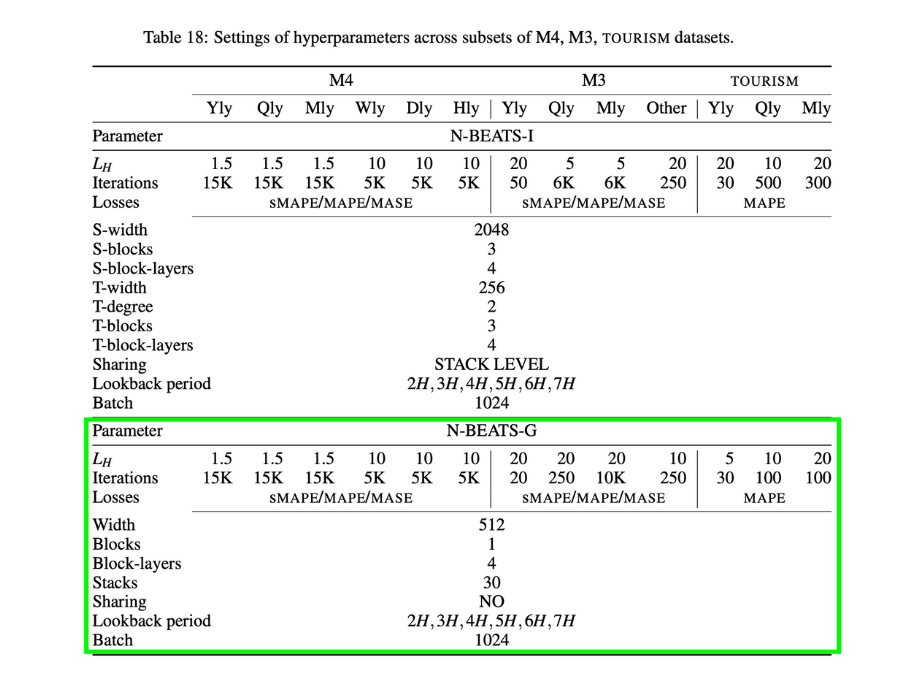
Source: Figure 1 and Table 18/Appendix D of the N-BEATS paper

In [ ]:

# Hyperparameters values different from the N-BEATS paper Figure 1 and Table 18/Appendix D

LOOKBACK = 7 # If I forecast to H-timesteps ahead, by how much factor should I lookback?
HORIZON = 1 # How much timesteps ahead I am interested to forecast?

N_EPOCHS = 5000
N_NEURONS = 512
N_LAYERS = 4
N_STACKS = 30
N_BLOCKS = 1

INPUT_SIZE = LOOKBACK*HORIZON
THETA_SIZE = LOOKBACK + HORIZON

INPUT_SIZE, THETA_SIZE
# Hyperparameters values different from the N-BEATS paper Figure 1 and Table 18/Appendix D

LOOKBACK = 7 # If I forecast to H-timesteps ahead, by how much factor should I lookback?
HORIZON = 1 # How much timesteps ahead I am interested to forecast?

N_EPOCHS = 5000
N_NEURONS = 512
N_LAYERS = 4
N_STACKS = 30
N_BLOCKS = 1

INPUT_SIZE = LOOKBACK*HORIZON
THETA_SIZE = LOOKBACK + HORIZON

INPUT_SIZE, THETA_SIZE

Out[ ]:

(7, 8)

Now that the hyperparameters are ready, we need to create one important part of the architechture -> double residual stacking (section 3.2 of the N-BEATS paper) using the tf.keras.layers.subtract and tf.keras.layers.add layers

In [ ]:

# Random features
tensor_1 = tf.range(10)
tensor_2 = tf.range(10) + 10

# Subtract
subtracted = tf.keras.layers.subtract([tensor_2, tensor_1])

# Add
added = tf.keras.layers.add([tensor_2, tensor_1])

print(f'Input tensors:\n tensor_1: {tensor_1.numpy()}\n tensor_2: {tensor_2.numpy()}\n')
print(f'Subtracted: {subtracted.numpy()}')
print(f'Added: {added.numpy()}')
# Random features
tensor_1 = tf.range(10)
tensor_2 = tf.range(10) + 10

# Subtract
subtracted = tf.keras.layers.subtract([tensor_2, tensor_1])

# Add
added = tf.keras.layers.add([tensor_2, tensor_1])

print(f'Input tensors:\n tensor_1: {tensor_1.numpy()}\n tensor_2: {tensor_2.numpy()}\n')
print(f'Subtracted: {subtracted.numpy()}')
print(f'Added: {added.numpy()}')

Input tensors:
 tensor_1: [0 1 2 3 4 5 6 7 8 9]
 tensor_2: [10 11 12 13 14 15 16 17 18 19]

Subtracted: [10 10 10 10 10 10 10 10 10 10]
Added: [10 12 14 16 18 20 22 24 26 28]

In [ ]:

model_name= f'NBeatsGeneric_W{WINDOW}H{HORIZON}'
model_name= f'NBeatsGeneric_W{WINDOW}H{HORIZON}'

Creating the `NBeats` Model¶

Here, the number of Blocks i.e. the NBeatsBlock is 1 for each stack, with each such block having 4 Block-layers. Now this forms part of a NBeatsStack which are listed as being 30 in number. So as per my understanding the model architecture is as follows:

The inputs are taken as model_inputs
Now this is passed to a NBeatsStack.
Inside the NBeatsStack, we have 1 NBeatsBlock i.e. Block=1
Inside each NBeatsBlock we have 4 FC layers i.e. Block-layers=4, each of which outputs a block residual (subtracted cumulatively) and a block forecast (aggregated cumulatively)
Finally the residual which is subtracted cumulatively is passed on to the next stack, while forecast which is aggregated cumulatively is aggregated for each stack (30 times)

In [ ]:

# Set up the stack input layer
model_inputs = layers.Input(shape=INPUT_SIZE, name='model_input')

# Set up a template block
template_block = NBeatsBlock(input_size=INPUT_SIZE, theta_size=THETA_SIZE,
                             horizon=HORIZON, n_neurons=N_NEURONS, n_layers=N_LAYERS)

# Set up the initial stack
initial_stack = NBeatsStack(template_block, n_blocks=N_BLOCKS, name='stack0')

# Get residuals and forecast from the initial stack
residuals, forecast =  initial_stack(model_inputs)

for stack_num in range(1, N_STACKS):
    stack = NBeatsStack(template_block, n_blocks=N_BLOCKS, name=f'stack{stack_num}')
    residuals, stack_forecast = stack(residuals)

    forecast = layers.add([forecast, stack_forecast], name=f'{stack.name}_add')


model = tf.keras.Model(inputs=model_inputs, outputs=forecast, name=model_name)

model.compile(loss='mae', optimizer=tf.keras.optimizers.RMSprop(learning_rate=0.001), metrics=['mse'])

model.summary()
# Set up the stack input layer
model_inputs = layers.Input(shape=INPUT_SIZE, name='model_input')

# Set up a template block
template_block = NBeatsBlock(input_size=INPUT_SIZE, theta_size=THETA_SIZE,
                             horizon=HORIZON, n_neurons=N_NEURONS, n_layers=N_LAYERS)

# Set up the initial stack
initial_stack = NBeatsStack(template_block, n_blocks=N_BLOCKS, name='stack0')

# Get residuals and forecast from the initial stack
residuals, forecast =  initial_stack(model_inputs)

for stack_num in range(1, N_STACKS):
    stack = NBeatsStack(template_block, n_blocks=N_BLOCKS, name=f'stack{stack_num}')
    residuals, stack_forecast = stack(residuals)

    forecast = layers.add([forecast, stack_forecast], name=f'{stack.name}_add')


model = tf.keras.Model(inputs=model_inputs, outputs=forecast, name=model_name)

model.compile(loss='mae', optimizer=tf.keras.optimizers.RMSprop(learning_rate=0.001), metrics=['mse'])

model.summary()

Model: "NBeatsGeneric_W7H1"
__________________________________________________________________________________________________
Layer (type)                    Output Shape         Param #     Connected to                     
==================================================================================================
model_input (InputLayer)        [(None, 7)]          0                                            
__________________________________________________________________________________________________
stack0 (NBeatsStack)            ((None, 7), (None, 1 0           model_input[0][0]                
__________________________________________________________________________________________________
stack1 (NBeatsStack)            ((None, 7), (None, 1 0           stack0[0][0]                     
__________________________________________________________________________________________________
stack1_add (Add)                (None, 1)            0           stack0[0][1]                     
                                                                 stack1[0][1]                     
__________________________________________________________________________________________________
stack2 (NBeatsStack)            ((None, 7), (None, 1 0           stack1[0][0]                     
__________________________________________________________________________________________________
stack2_add (Add)                (None, 1)            0           stack1_add[0][0]                 
                                                                 stack2[0][1]                     
__________________________________________________________________________________________________
stack3 (NBeatsStack)            ((None, 7), (None, 1 0           stack2[0][0]                     
__________________________________________________________________________________________________
stack3_add (Add)                (None, 1)            0           stack2_add[0][0]                 
                                                                 stack3[0][1]                     
__________________________________________________________________________________________________
stack4 (NBeatsStack)            ((None, 7), (None, 1 0           stack3[0][0]                     
__________________________________________________________________________________________________
stack4_add (Add)                (None, 1)            0           stack3_add[0][0]                 
                                                                 stack4[0][1]                     
__________________________________________________________________________________________________
stack5 (NBeatsStack)            ((None, 7), (None, 1 0           stack4[0][0]                     
__________________________________________________________________________________________________
stack5_add (Add)                (None, 1)            0           stack4_add[0][0]                 
                                                                 stack5[0][1]                     
__________________________________________________________________________________________________
stack6 (NBeatsStack)            ((None, 7), (None, 1 0           stack5[0][0]                     
__________________________________________________________________________________________________
stack6_add (Add)                (None, 1)            0           stack5_add[0][0]                 
                                                                 stack6[0][1]                     
__________________________________________________________________________________________________
stack7 (NBeatsStack)            ((None, 7), (None, 1 0           stack6[0][0]                     
__________________________________________________________________________________________________
stack7_add (Add)                (None, 1)            0           stack6_add[0][0]                 
                                                                 stack7[0][1]                     
__________________________________________________________________________________________________
stack8 (NBeatsStack)            ((None, 7), (None, 1 0           stack7[0][0]                     
__________________________________________________________________________________________________
stack8_add (Add)                (None, 1)            0           stack7_add[0][0]                 
                                                                 stack8[0][1]                     
__________________________________________________________________________________________________
stack9 (NBeatsStack)            ((None, 7), (None, 1 0           stack8[0][0]                     
__________________________________________________________________________________________________
stack9_add (Add)                (None, 1)            0           stack8_add[0][0]                 
                                                                 stack9[0][1]                     
__________________________________________________________________________________________________
stack10 (NBeatsStack)           ((None, 7), (None, 1 0           stack9[0][0]                     
__________________________________________________________________________________________________
stack10_add (Add)               (None, 1)            0           stack9_add[0][0]                 
                                                                 stack10[0][1]                    
__________________________________________________________________________________________________
stack11 (NBeatsStack)           ((None, 7), (None, 1 0           stack10[0][0]                    
__________________________________________________________________________________________________
stack11_add (Add)               (None, 1)            0           stack10_add[0][0]                
                                                                 stack11[0][1]                    
__________________________________________________________________________________________________
stack12 (NBeatsStack)           ((None, 7), (None, 1 0           stack11[0][0]                    
__________________________________________________________________________________________________
stack12_add (Add)               (None, 1)            0           stack11_add[0][0]                
                                                                 stack12[0][1]                    
__________________________________________________________________________________________________
stack13 (NBeatsStack)           ((None, 7), (None, 1 0           stack12[0][0]                    
__________________________________________________________________________________________________
stack13_add (Add)               (None, 1)            0           stack12_add[0][0]                
                                                                 stack13[0][1]                    
__________________________________________________________________________________________________
stack14 (NBeatsStack)           ((None, 7), (None, 1 0           stack13[0][0]                    
__________________________________________________________________________________________________
stack14_add (Add)               (None, 1)            0           stack13_add[0][0]                
                                                                 stack14[0][1]                    
__________________________________________________________________________________________________
stack15 (NBeatsStack)           ((None, 7), (None, 1 0           stack14[0][0]                    
__________________________________________________________________________________________________
stack15_add (Add)               (None, 1)            0           stack14_add[0][0]                
                                                                 stack15[0][1]                    
__________________________________________________________________________________________________
stack16 (NBeatsStack)           ((None, 7), (None, 1 0           stack15[0][0]                    
__________________________________________________________________________________________________
stack16_add (Add)               (None, 1)            0           stack15_add[0][0]                
                                                                 stack16[0][1]                    
__________________________________________________________________________________________________
stack17 (NBeatsStack)           ((None, 7), (None, 1 0           stack16[0][0]                    
__________________________________________________________________________________________________
stack17_add (Add)               (None, 1)            0           stack16_add[0][0]                
                                                                 stack17[0][1]                    
__________________________________________________________________________________________________
stack18 (NBeatsStack)           ((None, 7), (None, 1 0           stack17[0][0]                    
__________________________________________________________________________________________________
stack18_add (Add)               (None, 1)            0           stack17_add[0][0]                
                                                                 stack18[0][1]                    
__________________________________________________________________________________________________
stack19 (NBeatsStack)           ((None, 7), (None, 1 0           stack18[0][0]                    
__________________________________________________________________________________________________
stack19_add (Add)               (None, 1)            0           stack18_add[0][0]                
                                                                 stack19[0][1]                    
__________________________________________________________________________________________________
stack20 (NBeatsStack)           ((None, 7), (None, 1 0           stack19[0][0]                    
__________________________________________________________________________________________________
stack20_add (Add)               (None, 1)            0           stack19_add[0][0]                
                                                                 stack20[0][1]                    
__________________________________________________________________________________________________
stack21 (NBeatsStack)           ((None, 7), (None, 1 0           stack20[0][0]                    
__________________________________________________________________________________________________
stack21_add (Add)               (None, 1)            0           stack20_add[0][0]                
                                                                 stack21[0][1]                    
__________________________________________________________________________________________________
stack22 (NBeatsStack)           ((None, 7), (None, 1 0           stack21[0][0]                    
__________________________________________________________________________________________________
stack22_add (Add)               (None, 1)            0           stack21_add[0][0]                
                                                                 stack22[0][1]                    
__________________________________________________________________________________________________
stack23 (NBeatsStack)           ((None, 7), (None, 1 0           stack22[0][0]                    
__________________________________________________________________________________________________
stack23_add (Add)               (None, 1)            0           stack22_add[0][0]                
                                                                 stack23[0][1]                    
__________________________________________________________________________________________________
stack24 (NBeatsStack)           ((None, 7), (None, 1 0           stack23[0][0]                    
__________________________________________________________________________________________________
stack24_add (Add)               (None, 1)            0           stack23_add[0][0]                
                                                                 stack24[0][1]                    
__________________________________________________________________________________________________
stack25 (NBeatsStack)           ((None, 7), (None, 1 0           stack24[0][0]                    
__________________________________________________________________________________________________
stack25_add (Add)               (None, 1)            0           stack24_add[0][0]                
                                                                 stack25[0][1]                    
__________________________________________________________________________________________________
stack26 (NBeatsStack)           ((None, 7), (None, 1 0           stack25[0][0]                    
__________________________________________________________________________________________________
stack26_add (Add)               (None, 1)            0           stack25_add[0][0]                
                                                                 stack26[0][1]                    
__________________________________________________________________________________________________
stack27 (NBeatsStack)           ((None, 7), (None, 1 0           stack26[0][0]                    
__________________________________________________________________________________________________
stack27_add (Add)               (None, 1)            0           stack26_add[0][0]                
                                                                 stack27[0][1]                    
__________________________________________________________________________________________________
stack28 (NBeatsStack)           ((None, 7), (None, 1 0           stack27[0][0]                    
__________________________________________________________________________________________________
stack28_add (Add)               (None, 1)            0           stack27_add[0][0]                
                                                                 stack28[0][1]                    
__________________________________________________________________________________________________
stack29 (NBeatsStack)           ((None, 7), (None, 1 0           stack28[0][0]                    
__________________________________________________________________________________________________
stack29_add (Add)               (None, 1)            0           stack28_add[0][0]                
                                                                 stack29[0][1]                    
==================================================================================================
Total params: 0
Trainable params: 0
Non-trainable params: 0
__________________________________________________________________________________________________

In [ ]:

tf.random.set_seed(42)

# 1. Setup N-BEATS Block layer
nbeats_block_layer = NBeatsBlock(input_size=INPUT_SIZE,
                                 theta_size=THETA_SIZE,
                                 horizon=HORIZON,
                                 n_neurons=N_NEURONS,
                                 n_layers=N_LAYERS,
                                 name="InitialBlock")

# 2. Create input to stacks
stack_input = layers.Input(shape=(INPUT_SIZE), name="stack_input")

# 3. Create initial backcast and forecast input (backwards predictions are referred to as residuals in the paper)
residuals, forecast = nbeats_block_layer(stack_input)

# 4. Create stacks of blocks
for i, _ in enumerate(range(N_STACKS-1)): # first stack is already creted in (3)

  # 5. Use the NBeatsBlock to calculate the backcast as well as block forecast
  backcast, block_forecast = NBeatsBlock(
      input_size=INPUT_SIZE,
      theta_size=THETA_SIZE,
      horizon=HORIZON,
      n_neurons=N_NEURONS,
      n_layers=N_LAYERS,
      name=f"NBeatsBlock_{i}"
  )(residuals) # pass it in residuals (the backcast)

  # 6. Create the double residual stacking
  residuals = layers.subtract([residuals, backcast], name=f"subtract_{i}") 
  forecast = layers.add([forecast, block_forecast], name=f"add_{i}")

# 7. Put the stack model together
model = tf.keras.Model(inputs=stack_input, 
                         outputs=forecast, 
                         name=model_name)

# 8. Compile with MAE loss and Adam optimizer
model.compile(loss="mae",
                optimizer=tf.keras.optimizers.Adam(0.001),
                metrics=["mae", "mse"])
tf.random.set_seed(42)

# 1. Setup N-BEATS Block layer
nbeats_block_layer = NBeatsBlock(input_size=INPUT_SIZE,
                                 theta_size=THETA_SIZE,
                                 horizon=HORIZON,
                                 n_neurons=N_NEURONS,
                                 n_layers=N_LAYERS,
                                 name="InitialBlock")

# 2. Create input to stacks
stack_input = layers.Input(shape=(INPUT_SIZE), name="stack_input")

# 3. Create initial backcast and forecast input (backwards predictions are referred to as residuals in the paper)
residuals, forecast = nbeats_block_layer(stack_input)

# 4. Create stacks of blocks
for i, _ in enumerate(range(N_STACKS-1)): # first stack is already creted in (3)

  # 5. Use the NBeatsBlock to calculate the backcast as well as block forecast
  backcast, block_forecast = NBeatsBlock(
      input_size=INPUT_SIZE,
      theta_size=THETA_SIZE,
      horizon=HORIZON,
      n_neurons=N_NEURONS,
      n_layers=N_LAYERS,
      name=f"NBeatsBlock_{i}"
  )(residuals) # pass it in residuals (the backcast)

  # 6. Create the double residual stacking
  residuals = layers.subtract([residuals, backcast], name=f"subtract_{i}") 
  forecast = layers.add([forecast, block_forecast], name=f"add_{i}")

# 7. Put the stack model together
model = tf.keras.Model(inputs=stack_input, 
                         outputs=forecast, 
                         name=model_name)

# 8. Compile with MAE loss and Adam optimizer
model.compile(loss="mae",
                optimizer=tf.keras.optimizers.Adam(0.001),
                metrics=["mae", "mse"])

In [ ]:

model.summary()
model.summary()

Model: "NBeatsGeneric_W7H1"
__________________________________________________________________________________________________
Layer (type)                    Output Shape         Param #     Connected to                     
==================================================================================================
stack_input (InputLayer)        [(None, 7)]          0                                            
__________________________________________________________________________________________________
InitialBlock (NBeatsBlock)      ((None, 7), (None, 1 796168      stack_input[0][0]                
__________________________________________________________________________________________________
NBeatsBlock_0 (NBeatsBlock)     ((None, 7), (None, 1 796168      InitialBlock[0][0]               
__________________________________________________________________________________________________
subtract_0 (Subtract)           (None, 7)            0           InitialBlock[0][0]               
                                                                 NBeatsBlock_0[0][0]              
__________________________________________________________________________________________________
NBeatsBlock_1 (NBeatsBlock)     ((None, 7), (None, 1 796168      subtract_0[0][0]                 
__________________________________________________________________________________________________
subtract_1 (Subtract)           (None, 7)            0           subtract_0[0][0]                 
                                                                 NBeatsBlock_1[0][0]              
__________________________________________________________________________________________________
NBeatsBlock_2 (NBeatsBlock)     ((None, 7), (None, 1 796168      subtract_1[0][0]                 
__________________________________________________________________________________________________
subtract_2 (Subtract)           (None, 7)            0           subtract_1[0][0]                 
                                                                 NBeatsBlock_2[0][0]              
__________________________________________________________________________________________________
NBeatsBlock_3 (NBeatsBlock)     ((None, 7), (None, 1 796168      subtract_2[0][0]                 
__________________________________________________________________________________________________
subtract_3 (Subtract)           (None, 7)            0           subtract_2[0][0]                 
                                                                 NBeatsBlock_3[0][0]              
__________________________________________________________________________________________________
NBeatsBlock_4 (NBeatsBlock)     ((None, 7), (None, 1 796168      subtract_3[0][0]                 
__________________________________________________________________________________________________
subtract_4 (Subtract)           (None, 7)            0           subtract_3[0][0]                 
                                                                 NBeatsBlock_4[0][0]              
__________________________________________________________________________________________________
NBeatsBlock_5 (NBeatsBlock)     ((None, 7), (None, 1 796168      subtract_4[0][0]                 
__________________________________________________________________________________________________
subtract_5 (Subtract)           (None, 7)            0           subtract_4[0][0]                 
                                                                 NBeatsBlock_5[0][0]              
__________________________________________________________________________________________________
NBeatsBlock_6 (NBeatsBlock)     ((None, 7), (None, 1 796168      subtract_5[0][0]                 
__________________________________________________________________________________________________
subtract_6 (Subtract)           (None, 7)            0           subtract_5[0][0]                 
                                                                 NBeatsBlock_6[0][0]              
__________________________________________________________________________________________________
NBeatsBlock_7 (NBeatsBlock)     ((None, 7), (None, 1 796168      subtract_6[0][0]                 
__________________________________________________________________________________________________
subtract_7 (Subtract)           (None, 7)            0           subtract_6[0][0]                 
                                                                 NBeatsBlock_7[0][0]              
__________________________________________________________________________________________________
NBeatsBlock_8 (NBeatsBlock)     ((None, 7), (None, 1 796168      subtract_7[0][0]                 
__________________________________________________________________________________________________
subtract_8 (Subtract)           (None, 7)            0           subtract_7[0][0]                 
                                                                 NBeatsBlock_8[0][0]              
__________________________________________________________________________________________________
NBeatsBlock_9 (NBeatsBlock)     ((None, 7), (None, 1 796168      subtract_8[0][0]                 
__________________________________________________________________________________________________
subtract_9 (Subtract)           (None, 7)            0           subtract_8[0][0]                 
                                                                 NBeatsBlock_9[0][0]              
__________________________________________________________________________________________________
NBeatsBlock_10 (NBeatsBlock)    ((None, 7), (None, 1 796168      subtract_9[0][0]                 
__________________________________________________________________________________________________
subtract_10 (Subtract)          (None, 7)            0           subtract_9[0][0]                 
                                                                 NBeatsBlock_10[0][0]             
__________________________________________________________________________________________________
NBeatsBlock_11 (NBeatsBlock)    ((None, 7), (None, 1 796168      subtract_10[0][0]                
__________________________________________________________________________________________________
subtract_11 (Subtract)          (None, 7)            0           subtract_10[0][0]                
                                                                 NBeatsBlock_11[0][0]             
__________________________________________________________________________________________________
NBeatsBlock_12 (NBeatsBlock)    ((None, 7), (None, 1 796168      subtract_11[0][0]                
__________________________________________________________________________________________________
subtract_12 (Subtract)          (None, 7)            0           subtract_11[0][0]                
                                                                 NBeatsBlock_12[0][0]             
__________________________________________________________________________________________________
NBeatsBlock_13 (NBeatsBlock)    ((None, 7), (None, 1 796168      subtract_12[0][0]                
__________________________________________________________________________________________________
subtract_13 (Subtract)          (None, 7)            0           subtract_12[0][0]                
                                                                 NBeatsBlock_13[0][0]             
__________________________________________________________________________________________________
NBeatsBlock_14 (NBeatsBlock)    ((None, 7), (None, 1 796168      subtract_13[0][0]                
__________________________________________________________________________________________________
add_0 (Add)                     (None, 1)            0           InitialBlock[0][1]               
                                                                 NBeatsBlock_0[0][1]              
__________________________________________________________________________________________________
subtract_14 (Subtract)          (None, 7)            0           subtract_13[0][0]                
                                                                 NBeatsBlock_14[0][0]             
__________________________________________________________________________________________________
add_1 (Add)                     (None, 1)            0           add_0[0][0]                      
                                                                 NBeatsBlock_1[0][1]              
__________________________________________________________________________________________________
NBeatsBlock_15 (NBeatsBlock)    ((None, 7), (None, 1 796168      subtract_14[0][0]                
__________________________________________________________________________________________________
add_2 (Add)                     (None, 1)            0           add_1[0][0]                      
                                                                 NBeatsBlock_2[0][1]              
__________________________________________________________________________________________________
subtract_15 (Subtract)          (None, 7)            0           subtract_14[0][0]                
                                                                 NBeatsBlock_15[0][0]             
__________________________________________________________________________________________________
add_3 (Add)                     (None, 1)            0           add_2[0][0]                      
                                                                 NBeatsBlock_3[0][1]              
__________________________________________________________________________________________________
NBeatsBlock_16 (NBeatsBlock)    ((None, 7), (None, 1 796168      subtract_15[0][0]                
__________________________________________________________________________________________________
add_4 (Add)                     (None, 1)            0           add_3[0][0]                      
                                                                 NBeatsBlock_4[0][1]              
__________________________________________________________________________________________________
subtract_16 (Subtract)          (None, 7)            0           subtract_15[0][0]                
                                                                 NBeatsBlock_16[0][0]             
__________________________________________________________________________________________________
add_5 (Add)                     (None, 1)            0           add_4[0][0]                      
                                                                 NBeatsBlock_5[0][1]              
__________________________________________________________________________________________________
NBeatsBlock_17 (NBeatsBlock)    ((None, 7), (None, 1 796168      subtract_16[0][0]                
__________________________________________________________________________________________________
add_6 (Add)                     (None, 1)            0           add_5[0][0]                      
                                                                 NBeatsBlock_6[0][1]              
__________________________________________________________________________________________________
subtract_17 (Subtract)          (None, 7)            0           subtract_16[0][0]                
                                                                 NBeatsBlock_17[0][0]             
__________________________________________________________________________________________________
add_7 (Add)                     (None, 1)            0           add_6[0][0]                      
                                                                 NBeatsBlock_7[0][1]              
__________________________________________________________________________________________________
NBeatsBlock_18 (NBeatsBlock)    ((None, 7), (None, 1 796168      subtract_17[0][0]                
__________________________________________________________________________________________________
add_8 (Add)                     (None, 1)            0           add_7[0][0]                      
                                                                 NBeatsBlock_8[0][1]              
__________________________________________________________________________________________________
subtract_18 (Subtract)          (None, 7)            0           subtract_17[0][0]                
                                                                 NBeatsBlock_18[0][0]             
__________________________________________________________________________________________________
add_9 (Add)                     (None, 1)            0           add_8[0][0]                      
                                                                 NBeatsBlock_9[0][1]              
__________________________________________________________________________________________________
NBeatsBlock_19 (NBeatsBlock)    ((None, 7), (None, 1 796168      subtract_18[0][0]                
__________________________________________________________________________________________________
add_10 (Add)                    (None, 1)            0           add_9[0][0]                      
                                                                 NBeatsBlock_10[0][1]             
__________________________________________________________________________________________________
subtract_19 (Subtract)          (None, 7)            0           subtract_18[0][0]                
                                                                 NBeatsBlock_19[0][0]             
__________________________________________________________________________________________________
add_11 (Add)                    (None, 1)            0           add_10[0][0]                     
                                                                 NBeatsBlock_11[0][1]             
__________________________________________________________________________________________________
NBeatsBlock_20 (NBeatsBlock)    ((None, 7), (None, 1 796168      subtract_19[0][0]                
__________________________________________________________________________________________________
add_12 (Add)                    (None, 1)            0           add_11[0][0]                     
                                                                 NBeatsBlock_12[0][1]             
__________________________________________________________________________________________________
subtract_20 (Subtract)          (None, 7)            0           subtract_19[0][0]                
                                                                 NBeatsBlock_20[0][0]             
__________________________________________________________________________________________________
add_13 (Add)                    (None, 1)            0           add_12[0][0]                     
                                                                 NBeatsBlock_13[0][1]             
__________________________________________________________________________________________________
NBeatsBlock_21 (NBeatsBlock)    ((None, 7), (None, 1 796168      subtract_20[0][0]                
__________________________________________________________________________________________________
add_14 (Add)                    (None, 1)            0           add_13[0][0]                     
                                                                 NBeatsBlock_14[0][1]             
__________________________________________________________________________________________________
subtract_21 (Subtract)          (None, 7)            0           subtract_20[0][0]                
                                                                 NBeatsBlock_21[0][0]             
__________________________________________________________________________________________________
add_15 (Add)                    (None, 1)            0           add_14[0][0]                     
                                                                 NBeatsBlock_15[0][1]             
__________________________________________________________________________________________________
NBeatsBlock_22 (NBeatsBlock)    ((None, 7), (None, 1 796168      subtract_21[0][0]                
__________________________________________________________________________________________________
add_16 (Add)                    (None, 1)            0           add_15[0][0]                     
                                                                 NBeatsBlock_16[0][1]             
__________________________________________________________________________________________________
subtract_22 (Subtract)          (None, 7)            0           subtract_21[0][0]                
                                                                 NBeatsBlock_22[0][0]             
__________________________________________________________________________________________________
add_17 (Add)                    (None, 1)            0           add_16[0][0]                     
                                                                 NBeatsBlock_17[0][1]             
__________________________________________________________________________________________________
NBeatsBlock_23 (NBeatsBlock)    ((None, 7), (None, 1 796168      subtract_22[0][0]                
__________________________________________________________________________________________________
add_18 (Add)                    (None, 1)            0           add_17[0][0]                     
                                                                 NBeatsBlock_18[0][1]             
__________________________________________________________________________________________________
subtract_23 (Subtract)          (None, 7)            0           subtract_22[0][0]                
                                                                 NBeatsBlock_23[0][0]             
__________________________________________________________________________________________________
add_19 (Add)                    (None, 1)            0           add_18[0][0]                     
                                                                 NBeatsBlock_19[0][1]             
__________________________________________________________________________________________________
NBeatsBlock_24 (NBeatsBlock)    ((None, 7), (None, 1 796168      subtract_23[0][0]                
__________________________________________________________________________________________________
add_20 (Add)                    (None, 1)            0           add_19[0][0]                     
                                                                 NBeatsBlock_20[0][1]             
__________________________________________________________________________________________________
subtract_24 (Subtract)          (None, 7)            0           subtract_23[0][0]                
                                                                 NBeatsBlock_24[0][0]             
__________________________________________________________________________________________________
add_21 (Add)                    (None, 1)            0           add_20[0][0]                     
                                                                 NBeatsBlock_21[0][1]             
__________________________________________________________________________________________________
NBeatsBlock_25 (NBeatsBlock)    ((None, 7), (None, 1 796168      subtract_24[0][0]                
__________________________________________________________________________________________________
add_22 (Add)                    (None, 1)            0           add_21[0][0]                     
                                                                 NBeatsBlock_22[0][1]             
__________________________________________________________________________________________________
subtract_25 (Subtract)          (None, 7)            0           subtract_24[0][0]                
                                                                 NBeatsBlock_25[0][0]             
__________________________________________________________________________________________________
add_23 (Add)                    (None, 1)            0           add_22[0][0]                     
                                                                 NBeatsBlock_23[0][1]             
__________________________________________________________________________________________________
NBeatsBlock_26 (NBeatsBlock)    ((None, 7), (None, 1 796168      subtract_25[0][0]                
__________________________________________________________________________________________________
add_24 (Add)                    (None, 1)            0           add_23[0][0]                     
                                                                 NBeatsBlock_24[0][1]             
__________________________________________________________________________________________________
subtract_26 (Subtract)          (None, 7)            0           subtract_25[0][0]                
                                                                 NBeatsBlock_26[0][0]             
__________________________________________________________________________________________________
add_25 (Add)                    (None, 1)            0           add_24[0][0]                     
                                                                 NBeatsBlock_25[0][1]             
__________________________________________________________________________________________________
NBeatsBlock_27 (NBeatsBlock)    ((None, 7), (None, 1 796168      subtract_26[0][0]                
__________________________________________________________________________________________________
add_26 (Add)                    (None, 1)            0           add_25[0][0]                     
                                                                 NBeatsBlock_26[0][1]             
__________________________________________________________________________________________________
subtract_27 (Subtract)          (None, 7)            0           subtract_26[0][0]                
                                                                 NBeatsBlock_27[0][0]             
__________________________________________________________________________________________________
add_27 (Add)                    (None, 1)            0           add_26[0][0]                     
                                                                 NBeatsBlock_27[0][1]             
__________________________________________________________________________________________________
NBeatsBlock_28 (NBeatsBlock)    ((None, 7), (None, 1 796168      subtract_27[0][0]                
__________________________________________________________________________________________________
add_28 (Add)                    (None, 1)            0           add_27[0][0]                     
                                                                 NBeatsBlock_28[0][1]             
==================================================================================================
Total params: 23,885,040
Trainable params: 23,885,040
Non-trainable params: 0
__________________________________________________________________________________________________

Error: Solved here: https://stackoverflow.com/questions/58352326/running-the-tensorflow-2-0-code-gives-valueerror-tf-function-decorated-functio. I don't know how, but this solves it.

In [ ]:

tf.config.run_functions_eagerly(True)

tf.config.run_functions_eagerly(True)

In [ ]:

%%time

history = model.fit(train_tfdata, epochs=N_EPOCHS, validation_data=test_tfdata, verbose=0,
                    callbacks=[tf.keras.callbacks.EarlyStopping(monitor='val_loss', patience=200, restore_best_weights=True),
                               tf.keras.callbacks.ReduceLROnPlateau(monitor='val_loss', patience=100, verbose=1)])
%%time

history = model.fit(train_tfdata, epochs=N_EPOCHS, validation_data=test_tfdata, verbose=0,
                    callbacks=[tf.keras.callbacks.EarlyStopping(monitor='val_loss', patience=200, restore_best_weights=True),
                               tf.keras.callbacks.ReduceLROnPlateau(monitor='val_loss', patience=100, verbose=1)])

Epoch 01020: ReduceLROnPlateau reducing learning rate to 0.00010000000474974513.

Epoch 01445: ReduceLROnPlateau reducing learning rate to 1.0000000474974514e-05.

Epoch 01545: ReduceLROnPlateau reducing learning rate to 1.0000000656873453e-06.
CPU times: user 22min 52s, sys: 16.4 s, total: 23min 8s
Wall time: 22min 59s

In [ ]:

MODELS[model_name] = model
MODELS[model_name] = model

Learning Curve¶

In [ ]:

plot_learning_curve(model, extra_metric='mse', include_validation=True);
plot_learning_curve(model, extra_metric='mse', include_validation=True);

Why is there a spike in the learning curve? Hmm...

Way too heavily overfitted and noisy!

Make predictions¶

In [ ]:

preds = make_preds(model, test_tfdata)
preds.shape
preds = make_preds(model, test_tfdata)
preds.shape

Out[ ]:

TensorShape([564])

Evaluate predictions¶

In [ ]:

results = evaluate_preds(y_test, preds)
RESULTS[model_name] = results
results
results = evaluate_preds(y_test, preds)
RESULTS[model_name] = results
results

Out[ ]:

{'mae': array([657.32544], dtype=float32),
 'mape': array([0.02764818], dtype=float32),
 'mse': array([1393407.6], dtype=float32),
 'rmse': array([1180.4269], dtype=float32)}

In [ ]:

from tensorflow.keras.utils import plot_model as plot_keras_model
plot_keras_model(model, to_file='/tmp/model.png')
from tensorflow.keras.utils import plot_model as plot_keras_model
plot_keras_model(model, to_file='/tmp/model.png')

Out[ ]:

Model 8: Creating an ensemble (stacking different models together)¶

Ensembles which are uncorrelated (i.e. they are somewhat different learners), when combined often yield better result. This is the "decision of the crowd effect".
Ensembles win Kaggle competitions

In the N-BEATS paper, they trained an ensemble of models (180 in total, see section 3.4) to achieve the results they did using a combination of:

Different loss functions (sMAPE, MASE and MAPE)
Different window sizes (2 x horizon, 3 x horizon, 4 x horizon...)

But but but, sometimes due to the models being so big, and always being overfitted, due to the plethora of local minima present in the loss functions, even deep learning models with the same architechture with different random initilizations to their weights can produce different results

* This is a trick used by [Chris Deotte](https://www.kaggle.com/cdeotte) by setting different random seeds

We will create our ensemble as follows:

Using different loss functions (MAE, MSE, MAPE)
Randomly initializing the models
- Using a random normal distribution He normal initialization

In [ ]:

base_model = tf.keras.Sequential([
    layers.Dense(128, kernel_initializer='he_normal', activation='relu'),
    layers.Dense(128, kernel_initializer='he_normal', activation='relu'),
    layers.Dense(HORIZON)
], name='base_model')
base_model = tf.keras.Sequential([
    layers.Dense(128, kernel_initializer='he_normal', activation='relu'),
    layers.Dense(128, kernel_initializer='he_normal', activation='relu'),
    layers.Dense(HORIZON)
], name='base_model')

In [ ]:

def get_ensemble_models(base_model,train_data=train_tfdata, test_data=test_tfdata,
                        n_models=10, n_epochs=100, loss_funcs=['mae', 'mse', 'mape']):
    
    ensemble_models = []
    ensemble_predictions = []
    ensemble_results = []

    y_test = list(map(lambda x: x[1], test_data)) # Get target from PrefetchDataset

    for loss in loss_funcs:

        for i in range(1, n_models+1):

            model = tf.keras.models.clone_model(base_model)
            model._name = base_model.name + f'_{loss}{i}'
            model.compile(loss=loss, optimizer=tf.keras.optimizers.Adam(),
                            metrics=['mae', 'mse'])

            print(f'Training model with loss: {loss}, variant: {i}', end='\t')

            model.fit(train_data, validation_data=test_data, epochs=n_epochs, verbose=0,
                      callbacks=[tf.keras.callbacks.EarlyStopping(monitor='val_loss', patience=200, restore_best_weights=True),
                                 tf.keras.callbacks.ReduceLROnPlateau(monitor='val_loss', patience=100, verbose=0)])
            
            preds = make_preds(model, test_data)
            results = evaluate_preds(tf.squeeze(y_test), tf.squeeze(preds))

            s = []
            for metric, val in results.items():
                s.append(f'{metric} = {float(val):.2f}')

            print(', '.join(s))

            ensemble_models.append(model)
            ensemble_predictions.append(preds)
            ensemble_results.append(results)





    return ensemble_models, ensemble_predictions, ensemble_results
def get_ensemble_models(base_model,train_data=train_tfdata, test_data=test_tfdata,
                        n_models=10, n_epochs=100, loss_funcs=['mae', 'mse', 'mape']):
    
    ensemble_models = []
    ensemble_predictions = []
    ensemble_results = []

    y_test = list(map(lambda x: x[1], test_data)) # Get target from PrefetchDataset

    for loss in loss_funcs:

        for i in range(1, n_models+1):

            model = tf.keras.models.clone_model(base_model)
            model._name = base_model.name + f'_{loss}{i}'
            model.compile(loss=loss, optimizer=tf.keras.optimizers.Adam(),
                            metrics=['mae', 'mse'])

            print(f'Training model with loss: {loss}, variant: {i}', end='\t')

            model.fit(train_data, validation_data=test_data, epochs=n_epochs, verbose=0,
                      callbacks=[tf.keras.callbacks.EarlyStopping(monitor='val_loss', patience=200, restore_best_weights=True),
                                 tf.keras.callbacks.ReduceLROnPlateau(monitor='val_loss', patience=100, verbose=0)])
            
            preds = make_preds(model, test_data)
            results = evaluate_preds(tf.squeeze(y_test), tf.squeeze(preds))

            s = []
            for metric, val in results.items():
                s.append(f'{metric} = {float(val):.2f}')

            print(', '.join(s))

            ensemble_models.append(model)
            ensemble_predictions.append(preds)
            ensemble_results.append(results)





    return ensemble_models, ensemble_predictions, ensemble_results

In [ ]:

%%time
ensemble_models, ensemble_predictions, ensemble_results = get_ensemble_models(base_model, n_models=10, n_epochs=1000)
%%time
ensemble_models, ensemble_predictions, ensemble_results = get_ensemble_models(base_model, n_models=10, n_epochs=1000)

Training model with loss: mae, variant: 1	mae = 670.35, mse = 1435482.25, rmse = 1198.12, mape = 0.03
Training model with loss: mae, variant: 2	mae = 671.43, mse = 1465856.62, rmse = 1210.73, mape = 0.03
Training model with loss: mae, variant: 3	mae = 661.25, mse = 1445027.75, rmse = 1202.09, mape = 0.03
Training model with loss: mae, variant: 4	mae = 702.21, mse = 1536612.00, rmse = 1239.60, mape = 0.03
Training model with loss: mae, variant: 5	mae = 652.07, mse = 1424520.50, rmse = 1193.53, mape = 0.03
Training model with loss: mae, variant: 6	mae = 667.51, mse = 1452609.50, rmse = 1205.24, mape = 0.03
Training model with loss: mae, variant: 7	mae = 662.11, mse = 1429428.12, rmse = 1195.59, mape = 0.03
Training model with loss: mae, variant: 8	mae = 654.03, mse = 1364435.12, rmse = 1168.09, mape = 0.03
Training model with loss: mae, variant: 9	mae = 685.72, mse = 1528113.50, rmse = 1236.17, mape = 0.03
Training model with loss: mae, variant: 10	mae = 661.16, mse = 1421004.50, rmse = 1192.06, mape = 0.03
Training model with loss: mse, variant: 1	mae = 656.91, mse = 1419966.62, rmse = 1191.62, mape = 0.03
Training model with loss: mse, variant: 2	mae = 681.11, mse = 1476751.88, rmse = 1215.22, mape = 0.03
Training model with loss: mse, variant: 3	mae = 657.55, mse = 1386588.25, rmse = 1177.53, mape = 0.03
Training model with loss: mse, variant: 4	mae = 666.25, mse = 1391233.62, rmse = 1179.51, mape = 0.03
Training model with loss: mse, variant: 5	mae = 663.43, mse = 1423982.12, rmse = 1193.31, mape = 0.03
Training model with loss: mse, variant: 6	mae = 663.20, mse = 1425852.50, rmse = 1194.09, mape = 0.03
Training model with loss: mse, variant: 7	mae = 656.18, mse = 1415798.12, rmse = 1189.87, mape = 0.03
Training model with loss: mse, variant: 8	mae = 666.21, mse = 1425088.50, rmse = 1193.77, mape = 0.03
Training model with loss: mse, variant: 9	mae = 654.67, mse = 1381196.88, rmse = 1175.24, mape = 0.03
Training model with loss: mse, variant: 10	mae = 663.06, mse = 1405337.12, rmse = 1185.47, mape = 0.03
Training model with loss: mape, variant: 1	mae = 648.79, mse = 1380018.12, rmse = 1174.74, mape = 0.03
Training model with loss: mape, variant: 2	mae = 647.48, mse = 1388015.75, rmse = 1178.14, mape = 0.03
Training model with loss: mape, variant: 3	mae = 649.64, mse = 1385607.00, rmse = 1177.12, mape = 0.03
Training model with loss: mape, variant: 4	mae = 651.81, mse = 1373586.50, rmse = 1172.00, mape = 0.03
Training model with loss: mape, variant: 5	mae = 642.23, mse = 1359732.12, rmse = 1166.08, mape = 0.03
Training model with loss: mape, variant: 6	mae = 654.79, mse = 1384865.75, rmse = 1176.80, mape = 0.03
Training model with loss: mape, variant: 7	mae = 647.65, mse = 1361251.38, rmse = 1166.73, mape = 0.03
Training model with loss: mape, variant: 8	mae = 652.77, mse = 1394521.25, rmse = 1180.90, mape = 0.03
Training model with loss: mape, variant: 9	mae = 653.88, mse = 1381597.00, rmse = 1175.41, mape = 0.03
Training model with loss: mape, variant: 10	mae = 643.60, mse = 1344850.25, rmse = 1159.68, mape = 0.03
CPU times: user 29min 4s, sys: 1min 28s, total: 30min 33s
Wall time: 28min 47s

Ensemble mean¶

In [ ]:

ensemble_mean_results = evaluate_preds(y_test, np.mean(ensemble_predictions, axis=0))
ensemble_mean_results
ensemble_mean_results = evaluate_preds(y_test, np.mean(ensemble_predictions, axis=0))
ensemble_mean_results

Out[ ]:

{'mae': array([644.93396], dtype=float32),
 'mape': array([0.02686146], dtype=float32),
 'mse': array([1369131.6], dtype=float32),
 'rmse': array([1170.099], dtype=float32)}

Ensemble median¶

In [ ]:

ensemble_median_results = evaluate_preds(y_test, np.median(ensemble_predictions, axis=0))
ensemble_median_results
ensemble_median_results = evaluate_preds(y_test, np.median(ensemble_predictions, axis=0))
ensemble_median_results

Out[ ]:

{'mae': array([643.4394], dtype=float32),
 'mape': array([0.02665836], dtype=float32),
 'mse': array([1370662.8], dtype=float32),
 'rmse': array([1170.753], dtype=float32)}

In [ ]:

RESULTS['ensemble-mean_W7H1'] = ensemble_mean_results
RESULTS['ensemble-median_W7H1'] = ensemble_median_results
RESULTS['ensemble-mean_W7H1'] = ensemble_mean_results
RESULTS['ensemble-median_W7H1'] = ensemble_median_results

Plotting the prediction interval (quantifying ensemble uncertainty)¶

We are assuming the distribution of the ensemble predictions to be Gaussian. This may or may not be true (likely not true).

In [ ]:

import scipy
import scipy

Out[ ]:

1.959963984540054

In [ ]:

def get_confidence_interval(preds, conf=0.95):
    z_critical =  scipy.stats.norm.ppf(conf + (1-conf)/2)
    std = tf.math.reduce_std(preds, axis=0)
    interval = z_critical*std

    preds_mean = tf.reduce_mean(preds, axis=0)
    lower, upper = preds_mean - interval, preds_mean + interval

    return preds_mean, lower, upper
def get_confidence_interval(preds, conf=0.95):
    z_critical =  scipy.stats.norm.ppf(conf + (1-conf)/2)
    std = tf.math.reduce_std(preds, axis=0)
    interval = z_critical*std

    preds_mean = tf.reduce_mean(preds, axis=0)
    lower, upper = preds_mean - interval, preds_mean + interval

    return preds_mean, lower, upper

In [ ]:

preds_mean, lower, upper = get_confidence_interval(ensemble_predictions)
preds_mean, lower, upper = get_confidence_interval(ensemble_predictions)

In [ ]:

X_test.index
X_test.index

Out[ ]:

DatetimeIndex(['2019-12-09', '2019-12-10', '2019-12-11', '2019-12-12',
               '2019-12-13', '2019-12-14', '2019-12-15', '2019-12-16',
               '2019-12-17', '2019-12-18',
               ...
               '2021-06-15', '2021-06-16', '2021-06-17', '2021-06-18',
               '2021-06-19', '2021-06-20', '2021-06-21', '2021-06-22',
               '2021-06-23', '2021-06-24'],
              dtype='datetime64[ns]', name='date', length=564, freq=None)

In [ ]:

plt.figure(figsize=(12, 7))
offset = 500
plt.plot(X_test.index[offset:], y_test[offset:], 'g', label='test data')
plt.plot(X_test.index[offset:], preds_mean[offset:], 'k-', label='ensemble')

plt.fill_between(X_test.index[offset:],
                 lower[offset:],
                 upper[offset:], label='prediction interval')

plt.legend(fontsize=20)

plt.xlabel('Date')
plt.ylabel('BTC Price');
plt.figure(figsize=(12, 7))
offset = 500
plt.plot(X_test.index[offset:], y_test[offset:], 'g', label='test data')
plt.plot(X_test.index[offset:], preds_mean[offset:], 'k-', label='ensemble')

plt.fill_between(X_test.index[offset:],
                 lower[offset:],
                 upper[offset:], label='prediction interval')

plt.legend(fontsize=20)

plt.xlabel('Date')
plt.ylabel('BTC Price');

Oddly, it seems like model is lagging a bit in its predictions. The Daniel Bourke notebook mentions this maybe due to overfitting, but why would overfitting cause a lag in the predictions?

Model 9: Train a Dense model on the whole historical data to predict Bitcoin prices¶

After we make our artificial splits and find the best model, the final step is always to retrain the model on the whole data.

Note: Forecasting models need to be trained everytime a new prediction comes (maybe through retraining or online learning to adjust the weights). But care must always be taken to not spoil the model's weights just because of one highly unusual prediction (i.e. anomaly).

In [ ]:

bitcoin_prices_windowed.head()
bitcoin_prices_windowed.head()

Out[ ]:

	price	block_reward	price_lag1	price_lag2	price_lag3	price_lag4	price_lag5	price_lag6	price_lag7
date
2013-10-01	123.655	25.000	nan	nan	nan	nan	nan	nan	nan
2013-10-02	125.455	25.000	123.655	nan	nan	nan	nan	nan	nan
2013-10-03	108.585	25.000	125.455	123.655	nan	nan	nan	nan	nan
2013-10-04	118.675	25.000	108.585	125.455	123.655	nan	nan	nan	nan
2013-10-05	121.339	25.000	118.675	108.585	125.455	123.655	nan	nan	nan

In [ ]:

X_all = bitcoin_prices_windowed.drop(['price', 'block_reward'], axis=1).dropna().to_numpy()
y_all = bitcoin_prices_windowed['price'].to_numpy()
X_all = bitcoin_prices_windowed.drop(['price', 'block_reward'], axis=1).dropna().to_numpy()
y_all = bitcoin_prices_windowed['price'].to_numpy()

Great we have the $X$ and the $y$ now. Now we will prepare a dataset using the tf.data.Dataset API

In [ ]:

# Make feature and label tfdata
features_tfdata = tf.data.Dataset.from_tensor_slices(X_all)
labels_tfdata = tf.data.Dataset.from_tensor_slices(y_all)

# Zip them together
dataset_all = tf.data.Dataset.zip((features_tfdata, labels_tfdata))

# Batch and prefetch for optimal performance
BATCH_SIZE = 1024 # See Appendix D of N-Beats paper
dataset_all = dataset_all.batch(BATCH_SIZE).prefetch(buffer_size=tf.data.AUTOTUNE)

dataset_all
# Make feature and label tfdata
features_tfdata = tf.data.Dataset.from_tensor_slices(X_all)
labels_tfdata = tf.data.Dataset.from_tensor_slices(y_all)

# Zip them together
dataset_all = tf.data.Dataset.zip((features_tfdata, labels_tfdata))

# Batch and prefetch for optimal performance
BATCH_SIZE = 1024 # See Appendix D of N-Beats paper
dataset_all = dataset_all.batch(BATCH_SIZE).prefetch(buffer_size=tf.data.AUTOTUNE)

dataset_all

Out[ ]:

<PrefetchDataset shapes: ((None, 7), (None,)), types: (tf.float64, tf.float64)>

In [ ]:

model_name = 'dense-all-data_W7H1'
model_name = 'dense-all-data_W7H1'

In [ ]:

WINDOW = 7
HORIZON = 1
WINDOW = 7
HORIZON = 1

In [ ]:

tf.random.set_seed(42)

model = tf.keras.Sequential([
    layers.Dense(128, activation='relu', input_shape=(WINDOW,)),
    layers.Dense(128, activation='relu'),
    layers.Dense(HORIZON)
], name=model_name)

model.compile(loss='mae', optimizer=tf.keras.optimizers.Adam(), metrics=['mse'])

model.summary()
tf.random.set_seed(42)

model = tf.keras.Sequential([
    layers.Dense(128, activation='relu', input_shape=(WINDOW,)),
    layers.Dense(128, activation='relu'),
    layers.Dense(HORIZON)
], name=model_name)

model.compile(loss='mae', optimizer=tf.keras.optimizers.Adam(), metrics=['mse'])

model.summary()

Model: "dense-all-data_W7H1"
_________________________________________________________________
Layer (type)                 Output Shape              Param #   
=================================================================
dense_291704 (Dense)         (None, 128)               1024      
_________________________________________________________________
dense_291705 (Dense)         (None, 128)               16512     
_________________________________________________________________
dense_291706 (Dense)         (None, 1)                 129       
=================================================================
Total params: 17,665
Trainable params: 17,665
Non-trainable params: 0
_________________________________________________________________

In [ ]:

history = model.fit(dataset_all, epochs=100, verbose=0)
history = model.fit(dataset_all, epochs=100, verbose=0)

Learning Curve¶

In [ ]:

plot_learning_curve(history, extra_metric='mse');
plot_learning_curve(history, extra_metric='mse');

Predicting into the future¶

We will predict 14 days ahead into the future with our model with WINDOW=7, and HORIZON=1

In [ ]:

N_AHEAD = 14
N_AHEAD = 14

In [ ]:

def forecast_ahead_recursively(input_values, n_ahead, window_size, model):

    forecast = []
    last_window = input_values[-window_size:]

    for _ in range(n_ahead):
        pred = model.predict(tf.expand_dims(last_window, axis=0))
        forecast.append(tf.squeeze(pred).numpy())
        print(f'Predicting on window: {last_window} -> {tf.squeeze(pred).numpy()}\n')
        last_window = np.append(last_window, pred)[-window_size:]
    
    return forecast
def forecast_ahead_recursively(input_values, n_ahead, window_size, model):

    forecast = []
    last_window = input_values[-window_size:]

    for _ in range(n_ahead):
        pred = model.predict(tf.expand_dims(last_window, axis=0))
        forecast.append(tf.squeeze(pred).numpy())
        print(f'Predicting on window: {last_window} -> {tf.squeeze(pred).numpy()}\n')
        last_window = np.append(last_window, pred)[-window_size:]
    
    return forecast

In [ ]:

forecasts = forecast_ahead_recursively(y_all, n_ahead=N_AHEAD, window_size=7, model=model)
forecasts = forecast_ahead_recursively(y_all, n_ahead=N_AHEAD, window_size=7, model=model)

/usr/local/lib/python3.7/dist-packages/tensorflow/python/data/ops/dataset_ops.py:3704: UserWarning: Even though the `tf.config.experimental_run_functions_eagerly` option is set, this option does not apply to tf.data functions. To force eager execution of tf.data functions, please use `tf.data.experimental.enable.debug_mode()`.
  "Even though the `tf.config.experimental_run_functions_eagerly` "

Predicting on window: [37722.02018463 35520.45103404 35656.30473708 35681.13395636
 31659.54172976 32404.33035622 33532.25784581] -> 32636.619140625

Predicting on window: [35520.45103404 35656.30473708 35681.13395636 31659.54172976
 32404.33035622 33532.25784581 32636.61914062] -> 32201.40625

Predicting on window: [35656.30473708 35681.13395636 31659.54172976 32404.33035622
 33532.25784581 32636.61914062 32201.40625   ] -> 32116.45703125

Predicting on window: [35681.13395636 31659.54172976 32404.33035622 33532.25784581
 32636.61914062 32201.40625    32116.45703125] -> 32228.9921875

Predicting on window: [31659.54172976 32404.33035622 33532.25784581 32636.61914062
 32201.40625    32116.45703125 32228.9921875 ] -> 31990.830078125

Predicting on window: [32404.33035622 33532.25784581 32636.61914062 32201.40625
 32116.45703125 32228.9921875  31990.83007812] -> 31747.494140625

Predicting on window: [33532.25784581 32636.61914062 32201.40625    32116.45703125
 32228.9921875  31990.83007812 31747.49414062] -> 31682.65234375

Predicting on window: [32636.61914062 32201.40625    32116.45703125 32228.9921875
 31990.83007812 31747.49414062 31682.65234375] -> 31590.365234375

Predicting on window: [32201.40625    32116.45703125 32228.9921875  31990.83007812
 31747.49414062 31682.65234375 31590.36523438] -> 31450.38671875

Predicting on window: [32116.45703125 32228.9921875  31990.83007812 31747.49414062
 31682.65234375 31590.36523438 31450.38671875] -> 31308.4765625

Predicting on window: [32228.9921875  31990.83007812 31747.49414062 31682.65234375
 31590.36523438 31450.38671875 31308.4765625 ] -> 31202.412109375

Predicting on window: [31990.83007812 31747.49414062 31682.65234375 31590.36523438
 31450.38671875 31308.4765625  31202.41210938] -> 31093.3046875

Predicting on window: [31747.49414062 31682.65234375 31590.36523438 31450.38671875
 31308.4765625  31202.41210938 31093.3046875 ] -> 30968.29296875

Predicting on window: [31682.65234375 31590.36523438 31450.38671875 31308.4765625
 31202.41210938 31093.3046875  30968.29296875] -> 30848.626953125

Plot future forecasts¶

In [ ]:

def get_future_dates(start_date, n_ahead, offset=1):
    start_date = start_date + np.timedelta64(offset, 'D')
    end_date = start_date + np.timedelta64(n_ahead, 'D')

    return np.arange(start_date, end_date, dtype='datetime64[D]')
def get_future_dates(start_date, n_ahead, offset=1):
    start_date = start_date + np.timedelta64(offset, 'D')
    end_date = start_date + np.timedelta64(n_ahead, 'D')

    return np.arange(start_date, end_date, dtype='datetime64[D]')

In [ ]:

last_timestep = bitcoin_prices.index[-1]
last_timestep
last_timestep = bitcoin_prices.index[-1]
last_timestep

Out[ ]:

Timestamp('2021-06-24 00:00:00')

In [ ]:

forecast_timesteps = get_future_dates(start_date=last_timestep, n_ahead=N_AHEAD)
forecast_timesteps
forecast_timesteps = get_future_dates(start_date=last_timestep, n_ahead=N_AHEAD)
forecast_timesteps

Out[ ]:

array(['2021-06-25', '2021-06-26', '2021-06-27', '2021-06-28',
       '2021-06-29', '2021-06-30', '2021-07-01', '2021-07-02',
       '2021-07-03', '2021-07-04', '2021-07-05', '2021-07-06',
       '2021-07-07', '2021-07-08'], dtype='datetime64[D]')

Incorporate the last bitcoin prize into the forecast so that the plot doesn't break in the transition

In [ ]:

forecast_timesteps = np.insert(forecast_timesteps, 0, last_timestep)
forecasts = np.insert(forecasts, 0, bitcoin_prices['price'][-1])
forecast_timesteps = np.insert(forecast_timesteps, 0, last_timestep)
forecasts = np.insert(forecasts, 0, bitcoin_prices['price'][-1])

In [ ]:

plt.figure(figsize=(12, 7))
plot_bitcoin(bitcoin_prices.index, bitcoin_prices['price'], start=2700, linetype='-', label='BTC Price (historical)')
plot_bitcoin(forecast_timesteps, forecasts, linetype='-', label='BTC Price (forecasted)');
plt.xticks(rotation=45);
plt.figure(figsize=(12, 7))
plot_bitcoin(bitcoin_prices.index, bitcoin_prices['price'], start=2700, linetype='-', label='BTC Price (historical)')
plot_bitcoin(forecast_timesteps, forecasts, linetype='-', label='BTC Price (forecasted)');
plt.xticks(rotation=45);

Building a turkey model and why forecasting in an open system is BS¶

Introducing a Turkey problem to our BTC data (price BTC falls 100x in one day)

In [ ]:

btc_price_turkey = bitcoin_prices['price'].copy()
btc_price_turkey[-1] = btc_price_turkey[-1] / 100
btc_price_turkey = bitcoin_prices['price'].copy()
btc_price_turkey[-1] = btc_price_turkey[-1] / 100

In [ ]:

# Get the timesteps for the turkey problem 
btc_timesteps_turkey = np.array(bitcoin_prices.index)
btc_timesteps_turkey[-10:]
# Get the timesteps for the turkey problem 
btc_timesteps_turkey = np.array(bitcoin_prices.index)
btc_timesteps_turkey[-10:]

Out[ ]:

array(['2021-06-15T00:00:00.000000000', '2021-06-16T00:00:00.000000000',
       '2021-06-17T00:00:00.000000000', '2021-06-18T00:00:00.000000000',
       '2021-06-19T00:00:00.000000000', '2021-06-20T00:00:00.000000000',
       '2021-06-21T00:00:00.000000000', '2021-06-22T00:00:00.000000000',
       '2021-06-23T00:00:00.000000000', '2021-06-24T00:00:00.000000000'],
      dtype='datetime64[ns]')

Let's see how it looks

In [ ]:

plt.figure(figsize=(10, 7))
plot_bitcoin(tsteps=btc_timesteps_turkey, 
            prices=btc_price_turkey, 
            linetype="-", 
            label="BTC Price + Turkey Problem", 
            start=2500)
plt.figure(figsize=(10, 7))
plot_bitcoin(tsteps=btc_timesteps_turkey, 
            prices=btc_price_turkey, 
            linetype="-", 
            label="BTC Price + Turkey Problem", 
            start=2500)

Create train and test sets¶

In [ ]:

WINDOW = 7
HORIZON = 1
WINDOW = 7
HORIZON = 1

In [ ]:

# Create train and test sets for turkey problem data
full_windows, full_labels = make_window_horizon_pairs(np.array(btc_price_turkey), window=WINDOW, horizon=HORIZON)
len(full_windows), len(full_labels)

X_train, y_train, X_test, y_test = make_train_test_splits(full_windows, full_labels)
len(X_train), len(X_test)
# Create train and test sets for turkey problem data
full_windows, full_labels = make_window_horizon_pairs(np.array(btc_price_turkey), window=WINDOW, horizon=HORIZON)
len(full_windows), len(full_labels)

X_train, y_train, X_test, y_test = make_train_test_splits(full_windows, full_labels)
len(X_train), len(X_test)

Out[ ]:

(2252, 564)

In [ ]:

model_name = 'turkey-model_W7H1'
model_name = 'turkey-model_W7H1'

In [ ]:

turkey_model = tf.keras.models.clone_model(MODELS['simple-dense_W7H1'])
turkey_model._name = model_name
turkey_model.compile(loss='mae', optimizer=tf.keras.optimizers.Adam(), metrics=['mse'])
turkey_model.fit(X_train, y_train, epochs=100, verbose=0, validation_data=(X_test, y_test), callbacks=[create_model_checkpoint(model_name)])
turkey_model = tf.keras.models.clone_model(MODELS['simple-dense_W7H1'])
turkey_model._name = model_name
turkey_model.compile(loss='mae', optimizer=tf.keras.optimizers.Adam(), metrics=['mse'])
turkey_model.fit(X_train, y_train, epochs=100, verbose=0, validation_data=(X_test, y_test), callbacks=[create_model_checkpoint(model_name)])

/usr/local/lib/python3.7/dist-packages/tensorflow/python/data/ops/dataset_ops.py:3704: UserWarning: Even though the `tf.config.experimental_run_functions_eagerly` option is set, this option does not apply to tf.data functions. To force eager execution of tf.data functions, please use `tf.data.experimental.enable.debug_mode()`.
  "Even though the `tf.config.experimental_run_functions_eagerly` "

INFO:tensorflow:Assets written to: ../checkpoints/bitcoin_time_series_prediction/turkey-model_W7H1/assets
INFO:tensorflow:Assets written to: ../checkpoints/bitcoin_time_series_prediction/turkey-model_W7H1/assets
INFO:tensorflow:Assets written to: ../checkpoints/bitcoin_time_series_prediction/turkey-model_W7H1/assets
INFO:tensorflow:Assets written to: ../checkpoints/bitcoin_time_series_prediction/turkey-model_W7H1/assets
INFO:tensorflow:Assets written to: ../checkpoints/bitcoin_time_series_prediction/turkey-model_W7H1/assets
INFO:tensorflow:Assets written to: ../checkpoints/bitcoin_time_series_prediction/turkey-model_W7H1/assets
INFO:tensorflow:Assets written to: ../checkpoints/bitcoin_time_series_prediction/turkey-model_W7H1/assets
INFO:tensorflow:Assets written to: ../checkpoints/bitcoin_time_series_prediction/turkey-model_W7H1/assets
INFO:tensorflow:Assets written to: ../checkpoints/bitcoin_time_series_prediction/turkey-model_W7H1/assets
INFO:tensorflow:Assets written to: ../checkpoints/bitcoin_time_series_prediction/turkey-model_W7H1/assets
INFO:tensorflow:Assets written to: ../checkpoints/bitcoin_time_series_prediction/turkey-model_W7H1/assets
INFO:tensorflow:Assets written to: ../checkpoints/bitcoin_time_series_prediction/turkey-model_W7H1/assets
INFO:tensorflow:Assets written to: ../checkpoints/bitcoin_time_series_prediction/turkey-model_W7H1/assets
INFO:tensorflow:Assets written to: ../checkpoints/bitcoin_time_series_prediction/turkey-model_W7H1/assets
INFO:tensorflow:Assets written to: ../checkpoints/bitcoin_time_series_prediction/turkey-model_W7H1/assets

Out[ ]:

<tensorflow.python.keras.callbacks.History at 0x7f7febe11990>

Make predictions¶

In [ ]:

preds = make_preds(model, X_test)
preds.shape
preds = make_preds(model, X_test)
preds.shape

/usr/local/lib/python3.7/dist-packages/tensorflow/python/data/ops/dataset_ops.py:3704: UserWarning: Even though the `tf.config.experimental_run_functions_eagerly` option is set, this option does not apply to tf.data functions. To force eager execution of tf.data functions, please use `tf.data.experimental.enable.debug_mode()`.
  "Even though the `tf.config.experimental_run_functions_eagerly` "

Out[ ]:

TensorShape([564])

Evaluate predictions¶

In [ ]:

results = evaluate_preds(tf.squeeze(y_test), tf.squeeze(preds))
RESULTS[model_name] = results
results
results = evaluate_preds(tf.squeeze(y_test), tf.squeeze(preds))
RESULTS[model_name] = results
results

Out[ ]:

{'mae': array([780.02155], dtype=float32),
 'mape': array([0.19891468], dtype=float32),
 'mse': array([3393848.], dtype=float32),
 'rmse': array([1842.24], dtype=float32)}

In [ ]:

plt.figure(figsize=(12, 7))
offset=300
plot_bitcoin(tsteps=btc_timesteps_turkey[-len(X_test):], 
                 prices=btc_price_turkey[-len(y_test):], 
                 linetype="-", 
                 label="test data", start=offset)
plot_bitcoin(tsteps=btc_timesteps_turkey[-len(X_test):],
                 prices=preds, 
                 label="prediction", 
                 start=offset);

plt.title('Turkey Problem - Forecasting', fontdict=dict(weight='bold', size=20));
plt.figure(figsize=(12, 7))
offset=300
plot_bitcoin(tsteps=btc_timesteps_turkey[-len(X_test):], 
                 prices=btc_price_turkey[-len(y_test):], 
                 linetype="-", 
                 label="test data", start=offset)
plot_bitcoin(tsteps=btc_timesteps_turkey[-len(X_test):],
                 prices=preds, 
                 label="prediction", 
                 start=offset);

plt.title('Turkey Problem - Forecasting', fontdict=dict(weight='bold', size=20));

Beautiful image from `mrdbourke` illustrating the concept of Turkey problem | Black Swan Event¶

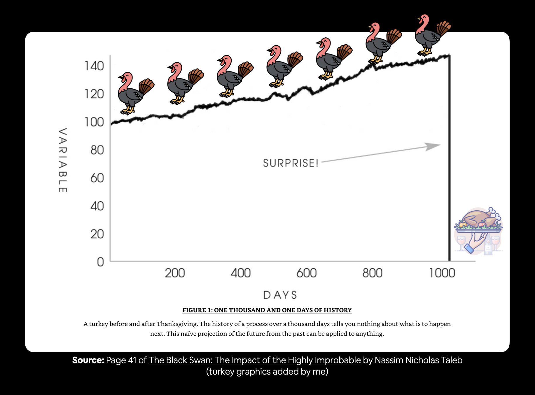
Compare model predictions¶

In [ ]:

result_df = pd.DataFrame(RESULTS)
result_df.applymap(_get_day1_pred).loc[['mae']].plot(figsize=(18, 7), kind='bar');
plt.title('Bitcoin time series forecasting', fontdict=dict(size=20, weight='bold'));
result_df = pd.DataFrame(RESULTS)
result_df.applymap(_get_day1_pred).loc[['mae']].plot(figsize=(18, 7), kind='bar');
plt.title('Bitcoin time series forecasting', fontdict=dict(size=20, weight='bold'));

Bitcoin Price Forecasting¶

Milestone Project 3¶

What is a time series problem?¶

Contents of this Notebook¶

Get the data¶

Change project directory¶

Components of a time series¶

Importing data using the Python's csv module¶

Formatting Data - 1. Creating training and tests sets the wrong way¶

2. Create train and test sets the right way¶

Modelling Experiments¶

Model 0: Naive Forecast (Baseline)¶

Evaluating a time series model¶

Scale-dependent errors¶¶

Percentage errors¶¶

Scaled errors¶¶

Various time series models which we can use for a baseline estimation¶

Formatting data - 2. Windowing the dataset¶

Turning windows into training and test sets¶

Make a modelling checkpoint¶

Function for easy training and reloading of KerasModel¶

Model 1: Dense Model (Window = 7, Horizon = 1)¶

Training function¶

Learning curve¶

Making forecasts with a time series model¶

Model 2: Dense (Window = 30, horizon = 1)¶

Make window-horizon pair dataset¶

Make train test splits¶

Learning curve¶

Get predictions¶

Evaluate the model¶

Model 3: Dense (Window = 30, horizon = 7)¶

Make window horizon pairs¶

Make train test splits¶

Make predictions¶

Evaluate the predictions¶

1-Day ahead forecast¶

2-Day ahead forecast¶

Which Dense model is performing best?¶

Model 4: Conv1D¶

Make window horizon pairs¶

Create train test splits¶

Create the model¶

Learning Curve¶

Make predictions¶

Evaluate predictions¶

Did our CNN model work well?¶

Model 5: LSTM¶

Make predictions¶

Evaluate predictions¶

Multivariate time series prediction¶

Make a windowed dataset for multivariate data¶

Model 6: Dense (multivariate time series)¶

Learning Curve¶

Make predictions¶

Evaluate predictions¶

Comparing model performance¶

Model 7: N-BEATS Algorithm¶

Building the N-BEATS block layer¶

Preparing data for the N-Beats algorithm using tf.Data¶

Setting up hyperparameters and extra layers for N-BEATS algorithm¶

Creating the NBeats Model¶

Learning Curve¶

Make predictions¶

Evaluate predictions¶

Model 8: Creating an ensemble (stacking different models together)¶

Ensemble mean¶

Ensemble median¶

Plotting the prediction interval (quantifying ensemble uncertainty)¶

Model 9: Train a Dense model on the whole historical data to predict Bitcoin prices¶

Learning Curve¶

Predicting into the future¶

Plot future forecasts¶

Building a turkey model and why forecasting in an open system is BS¶

Create train and test sets¶

Make predictions¶

Evaluate predictions¶

Beautiful image from mrdbourke illustrating the concept of Turkey problem | Black Swan Event¶

Compare model predictions¶

`Bitcoin Price Forecasting`¶

Importing data using the Python's `csv` module¶

Function for easy training and reloading of `KerasModel`¶

Preparing data for the N-Beats algorithm using `tf.Data`¶

Creating the `NBeats` Model¶

Beautiful image from `mrdbourke` illustrating the concept of Turkey problem | Black Swan Event¶